Win probability for football is simply the probability that a given team will win1 the game conditioned on the current state of the game. For instance when a team is up by two touchdowns late in the fourth quarter we want to give a quite high number say 98%. Conversely if it’s a very tight game you should give close to coin flips; and your model needs to react immediately. If you, in a completely hypothetical example decide not to run the ball with Marshawn Lynch and instead throw an interception on the goal line while slightly behind late in the game your win probability should immediately plummet from 85% to under 1%.
While obviously fun for fans (ESPN has a little ticker), it’s also useful for analytics. After all you’d like to measure plays based upon their impact on the team’s actual bottom line of winning games. You can think of this as the Moneyball-ification of football: it rewards the small unsexy plays that actually result in winning games.
Standard approaches fit regression models to observed win outcomes. This is fraught with difficulties stemming from the fact that you don’t get a lot of uncorrelated data to train on. There’s fewer than 300 NFL games a year and with rule changes and strategy shifts you don’t want to go back too far in time.
I, however, think there is a better way: simulation! Instead of having a ML model learn the intricate structure of football games you can embed that structure in a simulation leaving you free to spend your modelling budget capturing even more complicated structure. This, too, is fraught with difficulties but we’ll see that there’s also some advantages.
And just to cut to the chase: we see pretty similar prediction metrics relative to the standard NFLFastR models with much greater interpretability.
The series
This is the first of (at least) five posts:
- Simulating NFL Win Probability (this post) discusses the motivation and overview of the model.
- Inside the simulation model covers the details of the model architecture
- Win probability from fully synthetic data introduces the idea of using synthetic data to train our model
- Is it any good? Evaluating the model presents the results showing that we achieve pretty comparable performance to NFLFastR
- How much data does it need? uses our simulator as a source of ersatz data which we then use to make observations about win probability models in general
You can see predictions on historical games at the historical game browser. The code for the simulator is available on github.
Literature Review
There are two broad classes of prediction models: discriminative and generative.
Discriminative models are what we typically think of: they only model the quantity of interest \(E[Y \mid X]\). Most of the successful open-source win probability models are discriminative. Here’s a couple:
- Lock and Nettleton 2014: Random forests
- Yurko 2019 nflWAR: logistic regression for win probability
- NFLFastR extended the logistic regression into XGBoost and is the open-source baseline that we’ll compare our model against.
This is just a game of finding good features and fitting flexible off-the-shelf models.
Generative models on the other hand are more fiddly. They are interested in modelling the joint distribution \(P(X, Y)\). This seems relatively inefficient but typically (1) they’re easier to expand to distributions and (2) they let you impose structure in ways that are hard to do with discriminative models.
For football the primary structure is the fact that the game is a progression through state space as a Markov process. The idea of a state space model is not new: the oldest I can find is Goldner (2012) which treats (down, distance, yardline) as states of an absorbing Markov chain and solves for drive-ending / expected-point probabilities. Unfortunately doing this analytically blows up as you start adding state like clock dynamics which increase the size (and sparsity) of the states.
Thus the closest approach to what we’ll end up doing is Elmore, Williams 2021 with NFLSimulatoR which resamples plays to simulate drive. They use it to evaluate strategies (going for it on 4th down for instance). The main difference is that they model the drive (presumably because R is very very slow, making per-play infeasible).
Discriminative models typically beat generative models. The only hope for generative models is that they can encode information that discriminative models are not privy to: in particular structure.
Advantages of Simulation
Built-in Dynamics
So what is this structure that we want our simulation to capture? Consider the following scenario: you just went ahead by 2pts and are kicking off. How are you feeling?
If it’s early on in the game that’s pretty decent for you but not amazing: maybe 55-45 with lots of game left to play? But if it’s a few seconds to go you’re in pretty great shape at maybe 90%+! The reason for this is inherent to the rules of the game: there’s only so much time in the game and this constrains the outcomes. Similarly you’d be even happier if you were up by 9 points: the structure of scoring means that being up by 9 requires at least two possessions by the other team. And again time constrains the possibility of that happening. Note that I didn’t need any data to reach this conclusion.
These dynamics are all potentially learnable by our model. But what do they look like? Let’s look at the going ahead by 2pts situation: we know it’s meh at the start of the game and awesome in the last couple seconds. So is it a nice monotonic increase as time goes from early to late in the game?
Not at all. If we simulate the leading team’s win probability while varying only the time left (the trailing team receiving, first-and-ten at their own 25) we get a surprising curve. With only seconds on the clock the lead is nearly safe, as you’d expect. But this only happens late into the game with about two minutes left. Before then there’s just too much time left in the game: all sorts of things could happen.
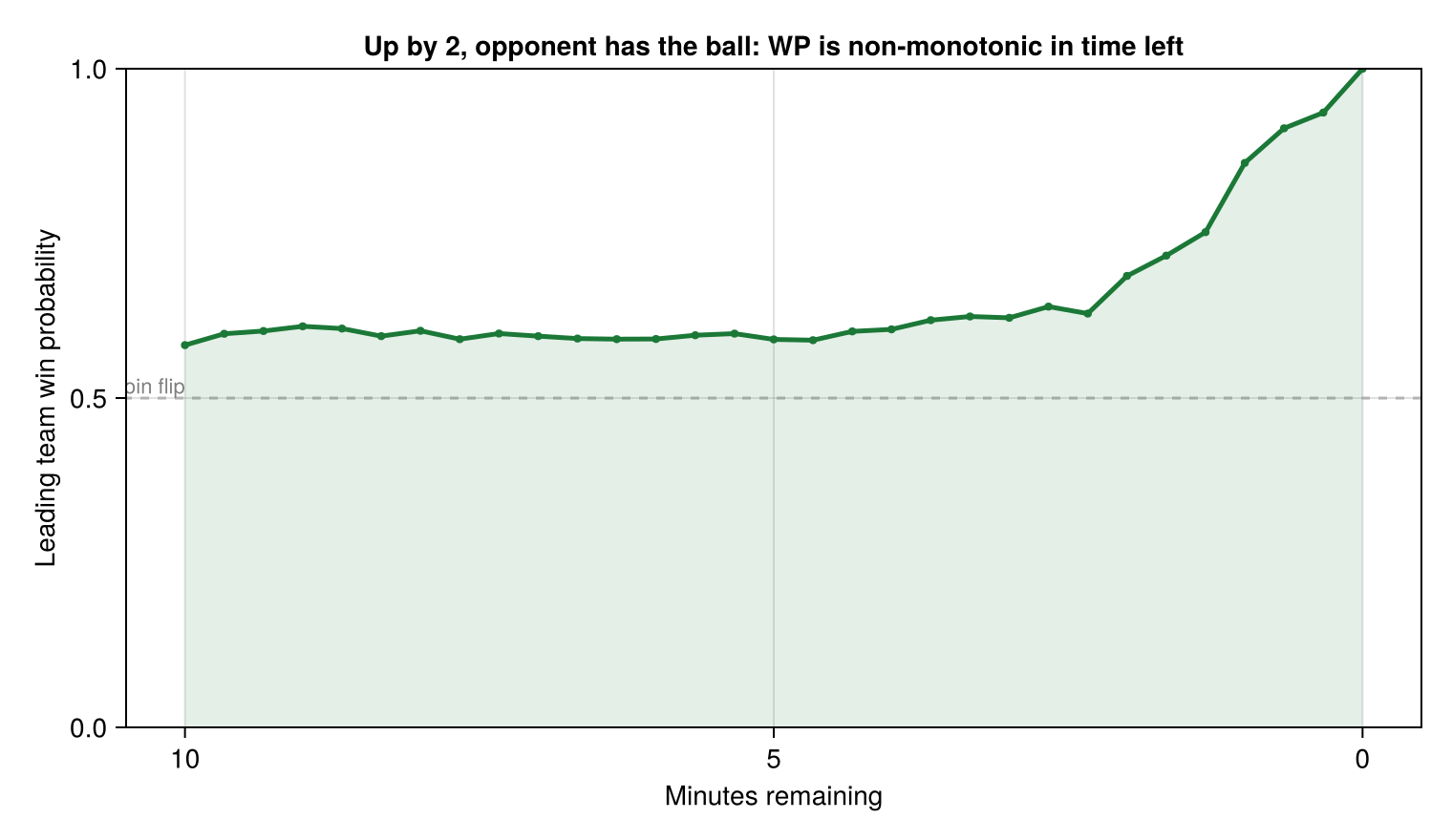
Figure 1: Win probability for the leading team (up by 2; first down for opponent at their own 25)
This is pretty tricky for a model to pick up. For instance, a linear model is infeasible 2. But even a highly flexible model will struggle with this as it really only applies when you’re up by two points late in the game. In the 2021-2025 era we see that there’s only 87 games where we end up in this situation: quite hard for a model to tease out such subtle changes in win probability.
Adaptable
It was surprising to me, a relative stranger to football, that it is not quite the same game as I remember as a child. Rules change and special circumstances arise all the time. For instance overtime is different between the regular season (where ties suck but can happen) and the post-season (one team must win). Then on top of that the rules have been changing: for instance in 2025 there’ve been changes to kickoff rules, touchbacks, and onside kicks as well as changes to the overtime rules.
How are we supposed to predict what’s going to happen in a game if the game is changing on us? The overtime change in particular has huge implications as both teams get a possession instead of sudden death where the first team can immediately win. If your model was trained on the old rules3 you’re going to be quite wrong in your predictions going forward. Indeed we can run these through our simulation and find that there’s a substantial change in the baseline advantage of going first as you go through the years. Though nicely it seems the NFL is iterating towards fairness.
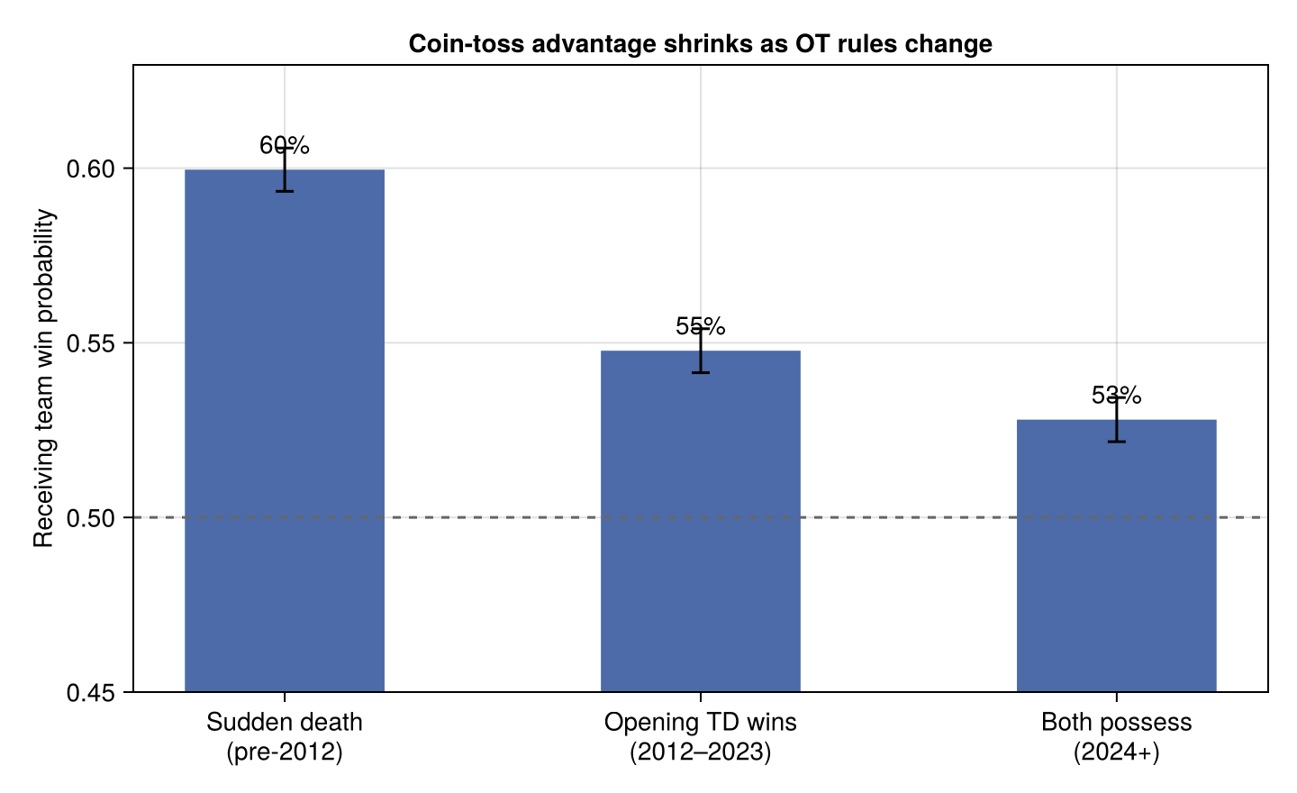
Overtime is a pretty big part of the game which has the virtue that, at the very least, you know that your model will be wrong with the overtime change. But what about more subtle changes? There’s apparently some talk of banning the tush push. If that happens it’s relatively straightforward to remove those plays from the simulator’s repertoire. But good luck trying to determine what, if any, effect this rule change will have on a ML model.
Interpretable
There’s a lot of implicit knowledge that we hold about football. One problem with blackbox win probability is that you don’t have a clear mechanism for improving the models. This ties back into the relatively minuscule, in ML terms, number of effective observations4. If you think the model is mispredicting in certain situations your only hope is replicating that situation many times.
Simulation, in contrast, provides trajectories: potential future paths that we can examine for plausibility. Instead of a blackbox prediction we can see why the prediction is the way that it is.
Let’s go back and examine the earlier scenario where a team goes up by 2 late in the game. Let’s look at the potential outcomes in two situations: with 2 minutes left and with 30 seconds left.
2 Minutes Remaining
30 Seconds Remaining
We can see the difference immediately. With 30 seconds left the trailing team’s tree is a thicket of dead ends: most rollouts simply run out the clock (or turn over the ball after going big) before they can reach field-goal range, so the leading team survives. Give them 2 minutes, though, and whole new branches open up: drives that reach a field goal to steal the lead, or even a touchdown because now there’s time for a real drive.
This visibility is rather important for debugging: you don’t need any ML knowledge to identify problems with simulated trajectories5. For instance, by looking at these sorts of graphs for an early version of the model, I found that teams were doing dumb things late in the game when trailing by spending way too much time in the huddle. I added a “urgency” feature to our play selection model which correctly modelled a sped-up offense.
Auxiliary Targets
Because we live in 2026 there are particular interests in several alternative summaries of the game.
For sports bettors this is the probability of beating the spread. This is hard to incorporate in a win probability model. Simple differencing of the scores approximates this: “count it as a win” if the team beats the spread. But typically teams are not trying to beat the spread; they just want to win. Thus your carefully honed endgame dynamics work against you: teams will strategically kick a field goal when down by 2 pts. But if they’re up and merely down by 2 relative to the spread they’re going to kneel the game over.
More respectably, there’s interest in expected points added which is the difference in expected points before and after the play. This is useful in advanced statistics to measure the efficiency of the offense accounting for the game situation. Naturally this is a different model than win probability though intuitively you’d suspect that both models should pick up on similar dynamics. Simulation however can provide estimates for both simultaneously (and self-consistently!).
We can have a little fun with this too and do some more outlandish stuff. Consider Scoregami which is a lovely concept popularized by Jon Bois. You should really watch the video, but to summarize, a scoregami is a game result which has never before been achieved in an NFL football game. Upon first glance this seems somewhat weird: we have a lot of football games, shouldn’t most scores have been achieved by now? But the unique structure of football with the counting by 2s, 3s, and 6s (and the resultant +1s, +2s) makes some scores rather hard to achieve 6. For instance getting 14 points is pretty easy: two touchdowns will get you there. But getting 5 points is pretty hard: the most straightforward route is a field goal and (a rare) safety and nothing else.
With our simulation we can predict whether a Scoregami will occur! This is a mess to do with a standard machine learning model (your target changes all the time and potentially even midgame!).
Counterfactual Decisions
A regression model can only tell you the win probability of the state you’re in. A simulator can answer a question that no amount of curve-fitting historical games can: what would the win probability be if the coach made a different choice on this play?
With a simulation we can force that action and then let the rest of the game unfold normally under the model. The gap between the choices is the value of that single decision.
You can even do this as a general rule. NFLSimulatoR, the R package that does the drive level simulation, does something similar by resampling historical plays, but it swaps out the strategy for entire drives.
Let’s consider an example: your down by 4 with 3:00 left at 4th-and-2 on your own yardline.
| Action | Home win probability |
|---|---|
| Run | 0.385 |
| Pass | 0.322 |
| Punt | 0.162 |
| Field goal | 0.141 |
The ordering the simulator returns is instructive: running it is clearly the best of the four. A pass is also pretty good though your chance of incompletions and interceptions stings a little. punt (though unrealistic) is then the next best and finally a fieldgoal doesn’t exactly help you too much.
I am somewhat skeptical of these results as they assume a stationarity of response. This is easiest to see with respect to trick plays. The analytics might tell you that the optimal approach is always to go with your trick play. But it really only works because they don’t see it coming; if you always did that play defenses would quickly adapt and shut you down. Adjusting your policy creates a follow-on adjustment that invalidates the expected gain.
You see this in broader contexts too. For instance, passing might be a better play but if you always pass then it becomes less efficient and thus you should put in some run plays7.
But unlike a discriminative model you can actually see this playing out! You have a model of what should happen and you can test it against what actually happens. If things are staying as expected you’re in good shape: otherwise caution.
This leads to the surprisingly inconspicuous elephant in the room of these sorts of analyses: the fact that the model is not entirely certain. This has been well articulated in the debate over whether to go for it on fourth down. I don’t really have any help here: if anything uncertainty quantification for the simulation is even harder than that for traditional ML models. But at least you can see it easier.
Challenges of Simulation
The Rules are Fiddly
I never realized how complicated the NFL’s rules were until I started coding them up. I challenge you to write down all of the various ways the play clock can be stopped. And don’t get me started on all the various rule changes over time.
Getting the simulator logic wrong can be pretty catastrophic. In an early version of the simulator I had terrible performance on a couple tight games because when the game clock expired I checked for overtime and otherwise ended the simulation. I completely forgot that if you score a touchdown as time expires you still get the PAT. So I had a ton of teams trailing by 6 or 7 who caught up with a touchdown but then my simulation didn’t allow them the easy +1 to tie or win the game.
If this was our only challenge however it wouldn’t be insurmountable. Just lots of careful bookkeeping and a robust test set. And some vibe coding to take away the tedium :)
You’ve got to be fast
A more daunting challenge is that you have to make the simulation fast! You’re going to running this code hundreds of thousands of times for each play: if it’s slow you’re just not going to be able to do it.
Fortunately the Julia language is well-suited for this task. We can achieve over 600,000 simulated plays per second on a cheap laptop: more than enough to provide a snappy in-game prediction.
We need more than just smart programming though: the choice of our model is important. For instance I tried an XGBoost-based model: this is pretty blazing fast amongst ML models. Too slow!! In the end I needed to make my own specialized CART trees to get fast enough. We’ll go into the details in the model post.
Modelling Play Distributions is Hard
This then leads to the crux of the problem: if we’re so limited with the models we can fit how can we possibly be expressive enough?
In particular we’re trying to model a probability distribution over plays. And we have to be clever about it: we don’t want to pick just any play. It wouldn’t do to randomly select a QB Kneel when we’re down by 2 in field goal range on the last play of the game. We want to sample the plays that match the historical games where the teams are in the same situation.
We also run into issues of censoring: if you’re on the 10 yard line by definition you can only gain 10 yards. But if you were way in the clear you might have run another 60 yards! That would be quite relevant for us when we’re considering what happens to that play at midfield. Though of course part of the reason why you would have run another 50 is because the short field negated deep coverage. Either way you cut it we have highly contextual dependencies on field location. Conditioning on the field location helps solve this: with 10-yard increments you can only be off by 9 yards, but that’s still particularly impactful in critical goal line scenarios.
Finally teams aren’t always consistent: in particular they respond to the strategic situation. We already discussed the ill-advised QB kneel situation. But this extends beyond play calling and into the outcomes. When teams are behind they tend to play more aggressively. Not accounting for this difference will lead to overstating the safety of leads.
I end up taking a two-stage approach. We use a very expensive model to estimate the play distribution but then distill it to our CART trees. For more details make sure to check out the post on the model and the post on the synthetic data.
Why are we doing all this
Before we go further into the details I want to address the natural criticism: there’s a bait and switch, we’re making conclusions about real football games but we’re only analyzing our simulated games. We know that our simulation does not capture the full dynamics of a football game. We could say the same thing about a more primitive version of our simulation or even a more advanced version. Is there some magical point at which we can trust that the simulation is fidelistic enough and we can for most purposes use it in lieu of real data? Or is this entire enterprise hopeless?
The standard statistical aphorism is “all models are wrong, but some are useful”. That said it’s a bit more of an art than a hard science. Simulations can elucidate key drivers: the hope is that by capturing the broad strokes of a system you’ll capture most of the relevant outcomes. This works in some circumstances: simulations are quite accurate for short-term weather prediction. But at the same time there are examples of systems which defy this logic: sometimes even the same system at different time scales. Those same weather simulations that work so well a few days in advance start failing if you start looking at them weeks out.
Thus it’s crucial to keep touch with reality when making conclusions with simulations. Often our real world data is messy and far too limited; but it can at least help to invalidate certain aspects of the simulation. In that vein I offer two rebuttals: firstly, empirically we seem to be doing pretty good in terms of predictions consistent with some good discriminative models. Two, if there’s a flaw in the simulation then that’s an opportunity for improvement. The visibility of model imperfections is simultaneously a reason to distrust it but also an opportunity to improve it8!
Ok, enough blabbering about statistical wisdom: let’s have some fun!
-
ignoring ties for now ↩︎
-
These dynamics are presumably why NFL FastR saw substantial benefits in moving away from logistic regressions to XGBoost ↩︎
-
You could technically train on playoff data which had the new ruleset, but then you’ve lost a good bit of data ↩︎
-
Remember that we actually have a lot of observations; it’s just that they’re all correlated so the effective number of independent observations is small. See the post on “How Much Data Does a Win-Probability Model Need?” (and its inspiration: “Exploring the Difficulty of Estimating Win Probability: A Simulation Study” by Brill, Yurko, and Wyner (2024)) ↩︎
-
though you’ll perhaps need that knowledge to fix it ↩︎
-
and hard to watch: just imagine the misery of watching a 2-2 tie ↩︎
-
There’s a great video about this regarding pass and run choices ↩︎
-
In particular, I currently don’t model penalties and have to introduce some heuristics for late-game decision making. Would appreciate PRs if you find an effective way to improve on this. ↩︎