Win Probability from Fully Synthetic Data

The limits of play-by-play data are many: it’s messy, it’s censored, and I just can’t get enough of it! To solve this problem I’d like to replace my real data with some synthetic data which avoids these problems.

Normalizing Flows

We’re currently working with CART trees to model our conditional distributions. To “sample” from the conditional distribution we’ll find the leaf corresponding to our covariates and then randomly sample one of the plays stored there.

An alternative approach to modelling (conditional) distributions is a (conditioned) normalizing flow. A normalizing flow is just a function which transforms one distribution into another distribution.

A transformed distribution can be determined by a base distribution and a bijector function f. As the name suggests the bijector is invertible and in particular it has a very nice inverse transformation with a very nice log determinant of the Jacobian. We can chain any number of invertible functions and the resulting function is still invertible thus we can make an entire neural network out of these functions which we’ll call the normalizing flow.

This lets us easily sample: just sample from the initial distribution and run it through the transform. We also get nice likelihoods: just take the original likelihood and scale it by the log determinant of the Jacobian.

To train this flow we start with a generic baseline distribution (usually a Normal for some reason). Then we simply do maximum likelihood estimation over the transformed distribution.

Now of course it’s way too slow to do this in our hot simulation loop. But we can do this as a preprocessing step: fit the normalizing flow on the real data and then generate a bunch of synthetic data from the model and fit our CART on top!

Adjusting for Censoring

Now why this indirection? We get some regularization from the model to smooth out our sparse real observations, but a more fundamental challenge is that the real distribution isn’t the right distribution!

The issue is censoring. When we’re running the simulation we draw plays in order to get a distribution over yards gained. Consider a touchdown: if we started on the 7 yard line we’d have a gain of 7 yards. But now say we drew that play when we’re on the 8 yard line: now no touchdown. But on the original play the guy could have probably made another yard: we just don’t record it because he crossed the goal line. Now I could condition on every yardline but that’s really causing too much sparsity.

The solution of course is to model this. When we see a touchdown we actually see a right-censored version of the underlying¹ play distribution. Thus we modify our loss function to accommodate: basically any value which satisfies the censoring constraint is equivalent to this loss.

\[ -\log \mathcal{L}(\theta) = -\!\!\sum_{i \,\in\, \text{observed}} \log f_\theta(y_i) \;-\!\!\sum_{j \,\in\, \text{censored}} \log\!\big(1 - F_\theta(c_j)\big), \]

where \(f_\theta\), \(F_\theta\) are the flow’s density and CDF of yards gained and \(c_j\) is the goal-line distance on censored touchdown \(j\).

Specializing our models to particular teams

Up until now we’ve been taking all of the data together. This is equivalent to simulating “generic” football teams. But we know that teams vary substantially in their performance.

We see this with the NFLFastR models: their Vegas model significantly outperforms their model which does not take team strength into consideration. The common finding within statistics is that you gain more from better data than better models. This holds true here: we need some way of incorporating what we know about teams into our simulation.

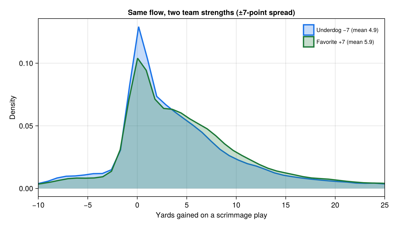
Fortunately this is just another covariate for our normalizing flow. We will have to learn two different distributions however: one for the Vegas favorite and one for the other team. As expected we’d see higher rates of gain for the favorite than the underdog.

using NFLWinProb
import NFLData

# Processed plays, plus the raw frame that carries the pregame Vegas line.
proc = NFLWinProb.get_play_by_play_data(2021:2023)
raw = NFLData.load_pbp(2021:2023)

# spread_cov: the pregame spread from the possessing offense's perspective — the
# same team-strength signal nflfastR's Vegas model uses.
team_df = attach_spread_covariate!(copy(proc), raw)

# One flow, now conditioned on that covariate.
gom = fit_generative_outcomes(team_df; covariate_cols = [:spread_cov])

# Same play contexts, two injected team strengths: a 7-point favorite vs underdog.
favorite = synth_corpus(gom, team_df; covariates = [+7.0])
underdog = synth_corpus(gom, team_df; covariates = [-7.0])