Inside the Simulation Model

Undertaking a simulation is a challenging task. You need to get a lot of fiddly details right. And you’re naturally oversimplifying a very complex situation.

Nevertheless all of the moving parts are roughly well contained and straightforward. We have the following components:

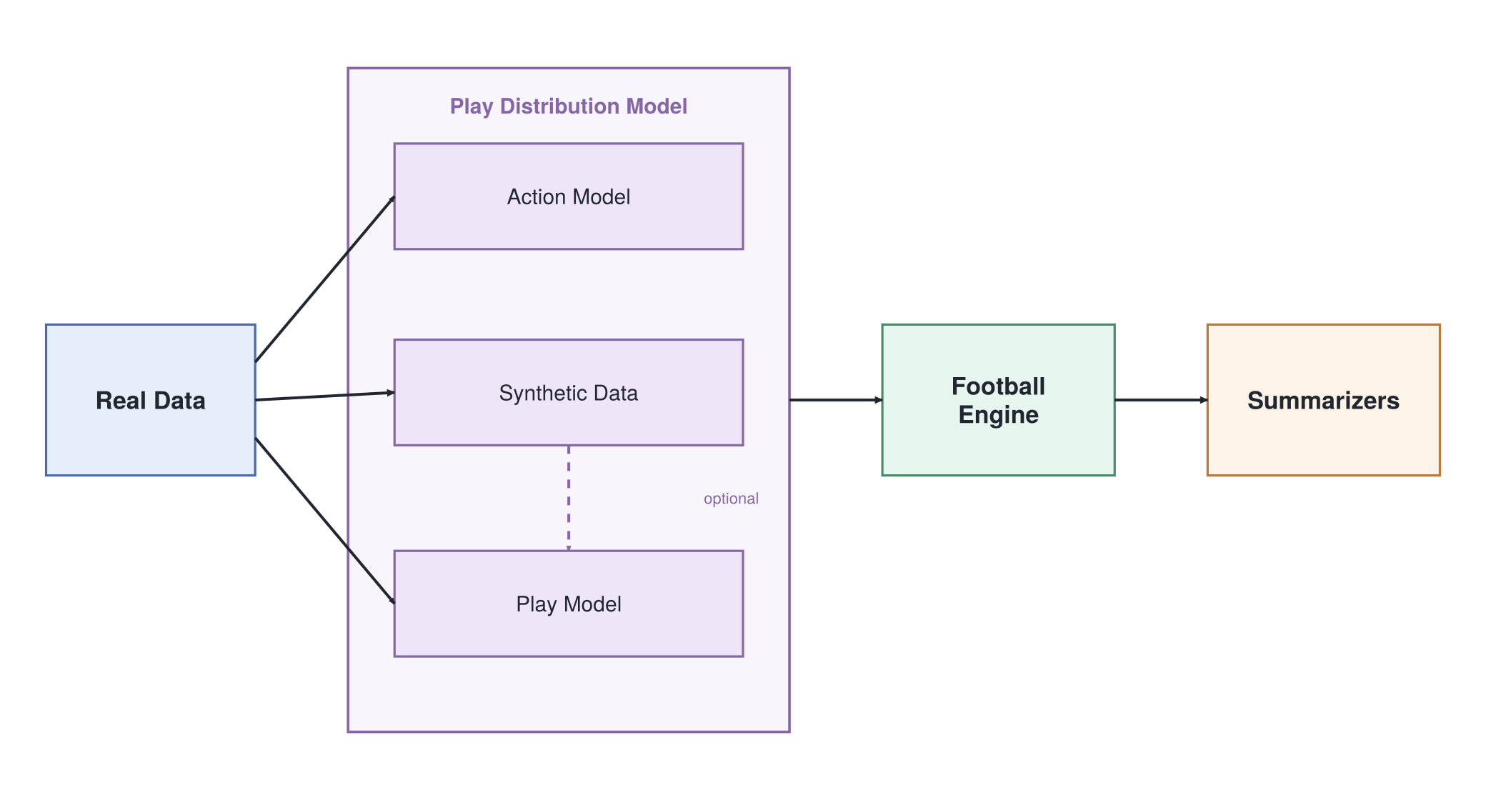
• The Play Distribution Model
  • The Action Model generates a random action based on the situation. This helps condition the set of possible plays.
  • The Synthetic Data Model (optional) replaces the true play data with an interpolated model to correct for censoring and fill out our play distribution.
  • The Play Model generates a random play based on the situation and the action.
• The Football Engine deterministically progresses the state of the game given the play.
• The Summarizers translate the simulations into quantities of interest such as win probability

The Data

The data comes from the NFLData package which is a wrapper for NFLFastR. They provide play-by-play data going back to 1999 although we’ll only use 2021 onwards (due to missingness for detailed play durations). We use this data extensively for both training and evaluation purposes.

The Play Distribution Model

We’ll separate the play selection into two parts: the action model (“Given this situation what will the team do?”) and the outcome model (“How does that go for them?”). We split them because we believe that play calls vary according to different covariates than play outcomes.

This is clearest with kickoffs: there’s a good deal of variation in deciding between kicking for returns, kicking out of the endzone, and having an onsides kick. That depends on the score differential, time left, and timeouts. But once you’ve decided to kick for return all that doesn’t really matter and the play will develop the way it is. By decoupling the action selection and the outcome we don’t force our models to share covariates and this in particular helps us aggregate play data (since modelling distributions is way harder than modelling action selection probabilities).

The Synthetic Data Model

I’m pulling this out into its own post as I need to introduce some heavier machinery. For now just understand that this takes in our covariates of game situation and action and returns a random play from the conditional play distribution.

You don’t actually have to have a model to do this. We could just return the original set of plays with no modelling whatsoever. This actually performs decently well though we find that further gains benefit greatly from fixing the sparsity and censoring problems inherent in the real data.

Simplifying our Models

The most pressing constraint on our models is that they have to be fast! They’re the inner loop of the game simulation so they’re going to be called for every play. Simulating a whole game from the start then has ~ 200 calls. We’ll continue to compute win probability on the subsequent plays: they are shorter though so it’s just (200 * 201) / 2 = 20100 calls total. And of course to reduce Monte Carlo noise we’ll run each simulation 1000 times yielding 20,100,000 calls per game.

Even if we were comfortable with full game simulations taking forever, for an in-game probability you’d like it to be as close to real time as possible. Thus we need 200,000 calls to take seconds (and remember that we need to save some time for the rest of the simulation). Thus our models need to be on the order of a microsecond.

This rules out a ton of models even seemingly blazing models like XGBoost which takes ~100 µs¹. And our usual tricks don’t help much. Batching? No: the simulation is an inherently linear process. Caching? No: the state space is way too big.

In the end the only model that worked fast enough was the humble decision tree. With our own implementation we can get over 600,000 plays per second on my dinky little laptop: just what we need. Note we can use trees for both the action selection and the outcome distribution. We just need a slight modification for the outcomes where we minimize the regression error of outcomes.

We needed our own implementation for three reasons:

Forced Splits

These are things that are hard to see from the data but which we want to split on. For instance we don’t want garbage time to infect the rest of the data so we split on that early in the tree. I also found that home field advantage wasn’t getting picked up in the model even though it compounds to a fairly large advantage and makes a substantial difference in the early game. It’s a legitimate criticism that a good model should actually pick these things up: however remember that CART is by-nature greedy and thus can’t make early splits that are slightly suboptimal in the moment but pay off further down the tree. This is our mechanism for helping it out a little.

Lazy Evaluation

We have a lot of features that we need to read in from the game state. But not all of them are needed for a single trip down the tree. If we had multiple trips it’d be fast to batch but we only use each state once! Thus to avoid doing any extra computation and more importantly allocation we have a lazy version which computes the requisite features on-the-fly as we go down the tree.

Leaf Storage

Unlike the usual library implementations of decision trees, we’re not interested in returning a point estimate. Instead we need to return a draw from a distribution. And the play distribution is pretty weird: you have lots of discontinuities and correlations. Simply storing some summary statistics at the end of the leaf and doing say a normal approximation wouldn’t be a good representation of the distribution we’re trying to represent. To get around this we do the simplest possible thing: we just use the empirical distribution! We store the indices of the training data which makes it into that leaf: then when we need to generate an observation we randomly select one of the indices from the leaf and return the corresponding play.

The Action Model

The action prediction stage is relatively straightforward. We can use the historical play-by-play data to learn the usual strategies of football teams. When they’re 4th and long in their own half they typically punt the ball. 3rd and inches from the goal is probably a running play.

We use the following features:

• Field location
• Down
• Yards to go
• Time left
• Score differential
• Time outs left

We then fit three models for each situation with corresponding valid playtypes

Regular Plays

[“run”, “pass”, “punt”, “fieldgoal”, “QB spike”, “QB kneel”, “offensive timeout”, “defensive timeout”].

Points After

[“1pt attempt”, “2pt attempt”]

Kickoffs

[“KickOutTheBack”, “KickForReturn”, “OnsidesKick”]

This is just a categorical regression so we use the usual gini loss for our CART splits. As you’ll see this buys us a lot: we don’t have to consider losses between different types of plays which have quite different representations.

Modelling Outcomes

After we have selected the action we need to determine the outcome: what results from the play? We need three bits of information: who has possession, where did the play end, and how much time did it take.

Note that the outcome differs depending on the action. For instance a run play results in a yardage change. A timeout clearly doesn’t. Because we have the action model we don’t have to model these two together. Indeed the timeout plays don’t even have a model: it’s just a deterministic outcome. Similarly field goals and points-after have their own specialized models which fit them parametrically since we have mostly binary outcomes.

It’s the run and pass plays which are complicated.

The main complication is correlation. Yards are not the only result of a play: the time taken is also crucial. Modelling time makes a big difference: the biggest jumps in performance came from me getting this right. A team that’s ahead is going to delay while a team that’s behind is going to play faster. And there’s all sorts of rules about when the clock runs and when it stops. And note the obvious fact: you make a 70 yard run it’s gonna take a lot longer than a stuffed qb sneak. Thus we need to model them jointly and that’s a bit of a mess.

To make our problem more tractable we actually decompose into three different outcomes: positive yardage, zero yardage, and negative yardage. These all have separate dynamics and thus we can learn them individually better than jointly. And it’s easy to do that by just keeping the plays intact as we receive them.

Thus when we fit our tree we actually cheat a little bit. We’re fitting a distribution over plays but we need some way of determining the split. We cheat and punt on getting a nice joint loss and just minimize a loss which considers the joint yards and time distribution². Empirically though it seems like it works nicely enough.

The Football Engine

This is the deterministic part of the simulation. Given a play’s outcome we just update our state space. We moved X yards taking Y seconds; this may trigger a first down so we reset the down and yards-to-go. If there’s a score we transition to the appropriate point-after situation.

To avoid crazy logic we make use of Julia’s multiple dispatch. Instead of lots of =if=s and =elseif=s we fit individual functions which dispatch on enumerations. This lets us work on small composable functions rather than a monolithic snarl.

The main functions we need to implement are:

• get_outcome(state, play) translates a state and a play into an outcome. Those being Touchdown, Safety, Touchback, Turnover, FirstDown, AfterPAT, FieldGoalResult, DefensiveTouchdown, TwoPointResult, KneelOutcome, SpikeOutcome, or TimeoutOutcome, and if you’re none of those just a RegularOutcome.
• update_state(state, outcome, play) takes the outcome and applies its update to the state.
• check_transitions cleans up the global game state so the other functions don’t have to consider things like halftime.

get_outcome()

Some of these are incredibly short: there’s really not much that can happen with a QB Kneel. On the contrary there’s a lot that can happen with a regular play from scrimmage: you could turn it over, you could score, you could get a first down, or maybe you just move down the field a little.

function get_outcome(state, ::QBSpike, play::Play)
    return SpikeOutcome()
end

function get_outcome(state, ::Union{RunPlay,PassPlay,NoHuddleRun,NoHuddlePass}, play::Play)
      new_location = state.location - play.yard_diff

      play.is_turnover && return new_location >= 100 ? DefensiveTouchdown() : Turnover()

      new_yards_to_go = state.yards_to_go - play.yard_diff

      new_location <= 0 && return Touchdown()
      new_location >= 100 && return Safety()
      new_yards_to_go <= 0 && return FirstDown()
      state.down >= 4 && return Turnover()
      return RegularOutcome()
  end

Note that we do not modify state at this point! While we have calculated the new location we actually delegate this to update_state!() so that we only have a single source of mutation and don’t have to reason about whether we’ve already updated the state.

update_state!()

Again note that some outcomes are more complicated than others. For instance with touchdowns we have to explicitly consider the overtime state. But because we’ve isolated the complexity to just this outcome we can keep other outcomes like the SpikeOutcome very straightforward. The key to not losing your mind understanding this flow is to enforce this separation of concerns as much as possible.

function update_state!(state::GameState, outcome::Touchdown, play)
    subtract_time!(state, play)
    update_score!(state, 6)

    # does this TD end OT? first poss: per ruleset; rebuttal (==2): if now leading; else always
    if state.in_overtime
        state.overtime_possession_count += 1
        ends = if state.overtime_possession_count < 2
            state.ot_rules.td_ends_game_on_first_possession
        elseif state.overtime_possession_count == 2
            ot_score_margin(state) > 0  # possession is still the scoring team
        else
            true
        end
        ends && end_overtime!(state)
          state.situation = ends ? ScrimmageSituation() : PointAfterSituation()
    else
        state.situation = PointAfterSituation()
    end

    state.location = 2 # Scrimmage at the 2-yard line (yardline_100 = 2)
    state.down = 1
    state.yards_to_go = 2
    state.clock_stopped = true
    return state
end

function update_state!(state::GameState, outcome::SpikeOutcome, play)
    subtract_time!(state, play)
    state.down += 1
    state.situation = ScrimmageSituation()
    state.clock_stopped = true # Spike stops clock
    return state
end

check_transitions

There is one piece of global context that we need to keep track of: the time. To avoid having to consider this for every single state update we break it out into its own function. This essentially checks whether we’ve blown past a time threshold (two-minute warning, halftime, or overtime) and updates the global state accordingly (with some specialization for overtime).

function check_transitions!(state::GameState, rng::AbstractRNG = Random.default_rng())
    state.situation isa PointAfterSituation && return false

    # 2:00 warning: first dead ball ≤2:00 stops the clock, once per half (resets re-arm it)
    if !state.two_minute_warning_given && state.time_left <= two_minute_mark(state)
        state.two_minute_warning_given = true
        state.clock_stopped = true
    end

    if !state.halftime_done && state.time_left <= 1800
        reset_halftime!(state)
        return true
    end

    if state.time_left <= 0 && state.home_score == state.away_score && !state.in_overtime
        if state.ot_rules.duration > 0
            reset_overtime!(state, rng)
            return true
        end
        state.in_overtime = true # If no OT, game ends as tie
    end

    return false
end

Summarizing the Game

With the machinery so far we can simulate the remainder of a game given a starting state. We then need to translate this into a win probability. This is quite simple: we go through our finished pseudo-games and record the final outcomes.

We achieve this with a callback with Summarizer objects. These are data structures which we run over game traces to, you know, summarize things. We have four functions:

• on_simulation_start!(summ, state) initializes the summarizer for a fresh simulation.
• on_step!(summ, state, play, outcome) updates the summarizer’s state in the middle of the simulation; this is needed for summarizers which are interested in quantities that aren’t visible from the final state (e.g. expected points, run yardage, etc).
• on_simulation_end!(summ, state) updates the summarizers state on simulation end. Usually this involves adding the results to a growing sum.
• value(summ) returns our final answer.

For instance win probability just needs on_simulation_end! as it only cares about the final score:

@kwdef mutable struct WinProbabilitySummarizer <: AbstractSummarizer
    home_wins::Int64 = 0
    ties::Int64 = 0
    count::Int64 = 0
end


function on_simulation_end!(summ::WinProbabilitySummarizer, state::GameState)
    summ.count += 1
    if state.home_score > state.away_score
        summ.home_wins += 1
    elseif state.home_score == state.away_score
        summ.ties += 1
    end
end

value(summ::WinProbabilitySummarizer) =
    summ.count == 0 ? 0.5 : (summ.home_wins + 0.5 * summ.ties) / summ.count

Expected points on the other hand requires the full gamut of functions:

  @kwdef mutable struct NextScoreEPSummarizer <: AbstractSummarizer
    total_points::Float64 = 0.0
    count::Int64 = 0
    start_possession::Int = 0
    start_home_score::Int = 0
    start_away_score::Int = 0
    start_halftime_done::Bool = false
    done::Bool = false
end

function _net_score(summ::NextScoreEPSummarizer, state::GameState)
    Δh = state.home_score - summ.start_home_score
    Δa = state.away_score - summ.start_away_score
    return summ.start_possession == HOME ? Float64(Δh - Δa) : Float64(Δa - Δh)
end

function on_simulation_start!(summ::NextScoreEPSummarizer, state::GameState)
    summ.start_possession = state.possession
    summ.start_home_score = state.home_score
    summ.start_away_score = state.away_score
    summ.start_halftime_done = state.halftime_done
    summ.done = false
end

function on_step!(
    summ::NextScoreEPSummarizer,
    state::GameState,
    play::Play,
    outcome::Outcome,
)
    summ.done && return

    if outcome isa Union{AfterPAT,TwoPointResult,FieldGoalResult,Safety}
        summ.total_points += _net_score(summ, state)
        summ.count += 1
        summ.done = true
        return
    end

    # Half ended with no score → next-score-in-half is 0
    if state.halftime_done != summ.start_halftime_done
        summ.total_points += 0.0
        summ.count += 1
        summ.done = true
    end
end

function on_simulation_end!(summ::NextScoreEPSummarizer, state::GameState)
    summ.done && return
    summ.total_points += 0.0
    summ.count += 1
end

value(summ::NextScoreEPSummarizer) = summ.total_points / summ.count

This setup is remarkably flexible. We can even use this to extract full play-by-play data from simulated games to study in their own right (see our post on How Much Data Does a Win Probability Model Need).

Bringing it all together

Thus the final simulation loop is actually quite straightforward

function simulate(
    state::GameState,
    play_generator,
    summarizers_raw...;
    action_generator,
    n_sims = 1,
    rng::AbstractRNG = Random.default_rng(),
)
    summarizers = SummarizerGroup(summarizers_raw)
    for _ in 1:n_sims
        notify!(summarizers, on_simulation_start!, state)
        st = copy(state)

        steps = 0
        while true
            steps >= MAX_STEPS &&
                error("> $MAX_STEPS steps in simulation: probable infinite loop")
            is_final_state(st) && break
            action = select_action(st, action_generator, rng)
            _advance!(st, action, play_generator, rng, summarizers) # fn barrier to keep action concrete
            steps += 1
        end

        notify!(summarizers, on_simulation_end!, st)
    end
    return summarizers_raw
end

function _advance!(state::GameState, action, generator, rng, summarizers)
    play = generate_play(state, action, generator, rng)
    outcome = get_outcome(state, play)
    update_state!(state, outcome, play)
    check_transitions!(state, rng)
    notify!(summarizers, on_step!, state, play, outcome)
end