Brill, Yurko, and Wyner (2024) make the point in “Exploring the Difficulty of Estimating Win Probability: A Simulation Study” that it’s actually quite hard to estimate win probability models. In particular they demonstrate that win probability models have much higher variance than you would otherwise suspect due to the correlated nature of the observations.
They show this with a very simplified random walk version of football. They calculate the effective sample size: the amount of independent data that would give equivalent performance finding it’s a significant shrinkage. And they leave us with the observation that “real American football is exponentially more complex than random walk football. Its game-state space is much larger, so we expect the ESS to be even smaller in real life”. Which naturally provokes the question: how much smaller should we expect?
We have a similar question which is “how much more data would be helpful”? Even with correlated data we can get enough to estimate well. But we are heavily limited because there’s only so many football seasons (at least with data).
However, with a ready source of simulated games we can start trying to answer both of these questions.
Data
Simulating an entire game is relatively easy: we just run the simulation once from the initial kickoff. A data-collection summarizer (see the model post for a recap) records every state along the way and writes it out in the same play-by-play schema we use for model fitting.
The crucial advantage over real football is that we know the true win probability at every state: it’s the simulation’s own generative process. We recover it by running many fresh rollouts from each state and recording the fraction the home team wins, then store it alongside the realized outcome. This lets us measure calibration directly and, later, read off the best score any model could possibly achieve.
The generator is a short loop over the simulator: simulate a game with the production generators, then re-roll each state many times for its true WP (~=PBPCollector= and build_row are the schema plumbing, in the analysis library):
With this data we can fit our win probability models over many different subsets of the data. We’ll focus on three:
- Our simulation model (refit on each subset of games).
- The XGBoost specification used by nflfastR, as discussed in the previous eval post.
- The true win probability itself, fed straight through as a “model”. This is a perfect predictor whose only error is the irreducible noise
Variance of Estimates
Let’s consider the sampling distribution of our predictions under the current amount of data:
We’ll split the data into many different “seasons” (random subsets of 300 games), refit the XGBoost and simulation models on each, and the record what each predicts for a few fixed game states. The spread across seasons is the sampling uncertainty. The dashed line marks the true win probability at that state for a sense of the bias.
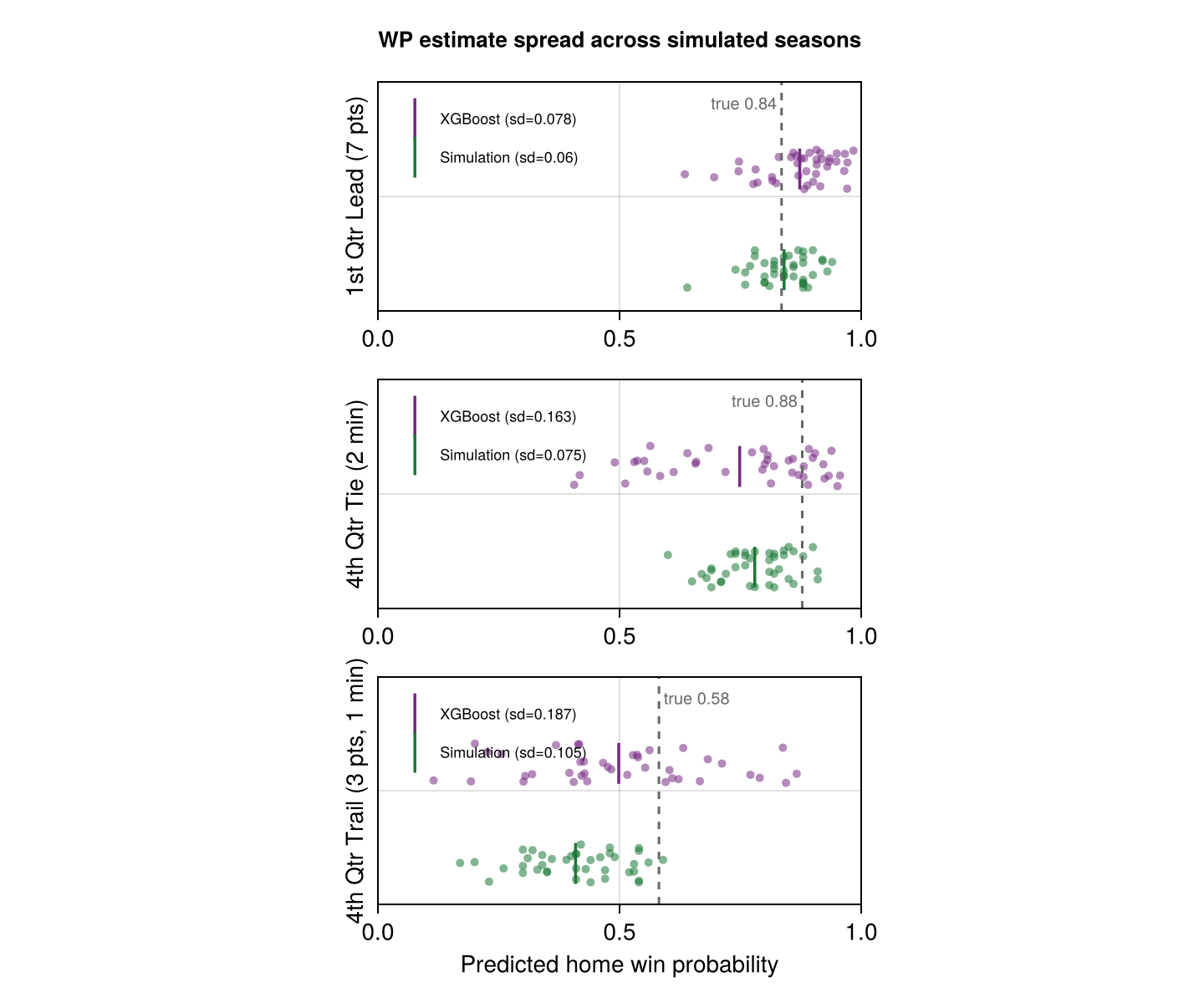
What we notice is that the variance of the estimate is actually quite dynamic. This is exactly what you would expect: the beginning of the game has a ton of data: every single game starts off in basically the same place! This branches off substantially in the late game where only a few games will reach these states. This leads to a correspondingly wide distribution for the predictions. I’m struck in particular by the final estimate where the distribution of probabilities almost span the whole range for XGBoost!
Note that the simulation’s spread is quite a bit tighter. This is indicative of a bias-variance tradeoff: the simulation is relatively low variance but as performance isn’t that much better it’s obvious that there’s a significant amount of bias. Even with infinite data the imperfections of our simulation will always be there.
The XGBoost model is the mirror image: it’s unbiased (asymptotically) but requires many samples to learn the nuances of the true win probability.
Thus we should see the simulation dominating when games are scarce and XGBoost catching up. Now with our particular setup it’ll never exceed the simulation: we actually have no structural bias against this particular synthetic data because, by construction, it comes from the simulation itself.
So how do these spreads translate into actual predictive loss as the data grows?
Performance curve
We can see this by fitting each model on increasing amounts of data and evaluating its Brier score on held-out games.
On synthetic data
Because we know the true win probability, we can draw the irreducible error: the Brier score you’d get from a perfect model, which is just the noise from games that could have gone either way. Every real model has to have loss above this.
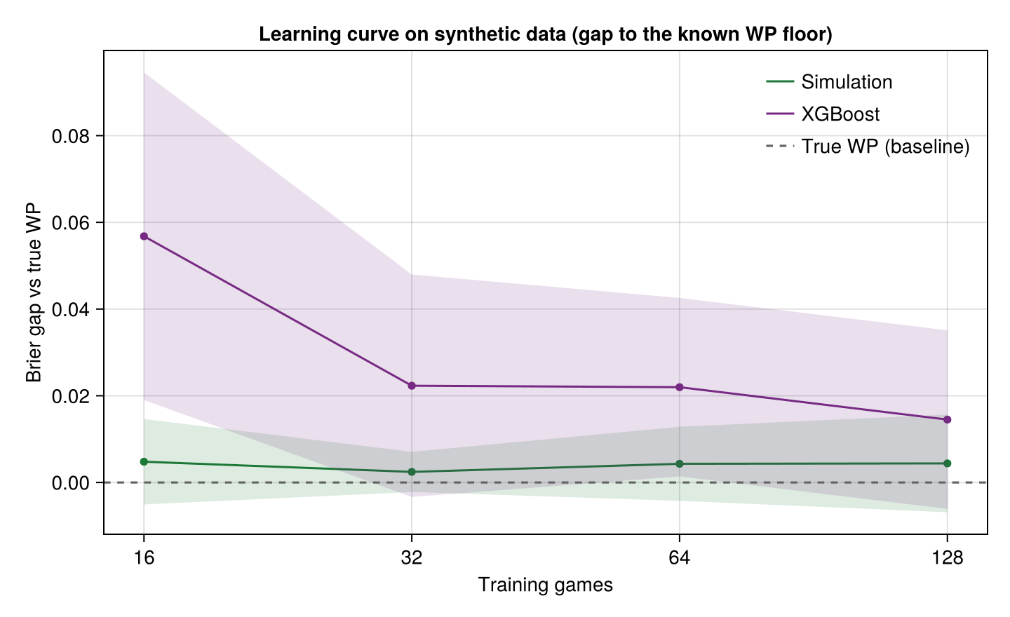
Thus we see the evolution. The simulation is pinned pretty closely to the floor while XGBoost starts much further away.
But we can look further. For instance in aggregate the simulation is statistically indistinguishable from optimal from the very first handful of games. This is wild and indeed the dumb model also does reasonably well.
The reason is that the well-sampled states that dominate the average are the ones it nails, and the sparse late-game wobble we just saw is too rare to move the mean. The answer is that Brier is a play-weighted average, and the plays are not created equal. Most states a game passes through are easy (say the opening kickoff where win probability is near 0.5 (modulo home-field advantage) for everyone), or the garbage-time downs of a blowout (near 0 or 1). Lots of games visit them, so they are at once the best-sampled states and the lowest-error ones, and they dominate the mean. The states we actually need a win probability model for (a one-score game in the final minutes) are rarer and get hidden in the average.
We can see this in a plot of the true win probability against each model’s prediction. Points on the dashed diagonal are perfect; vertical distance from it is error. We’ll also highlight these rarer tighter games coloring in games which are within a field goal.
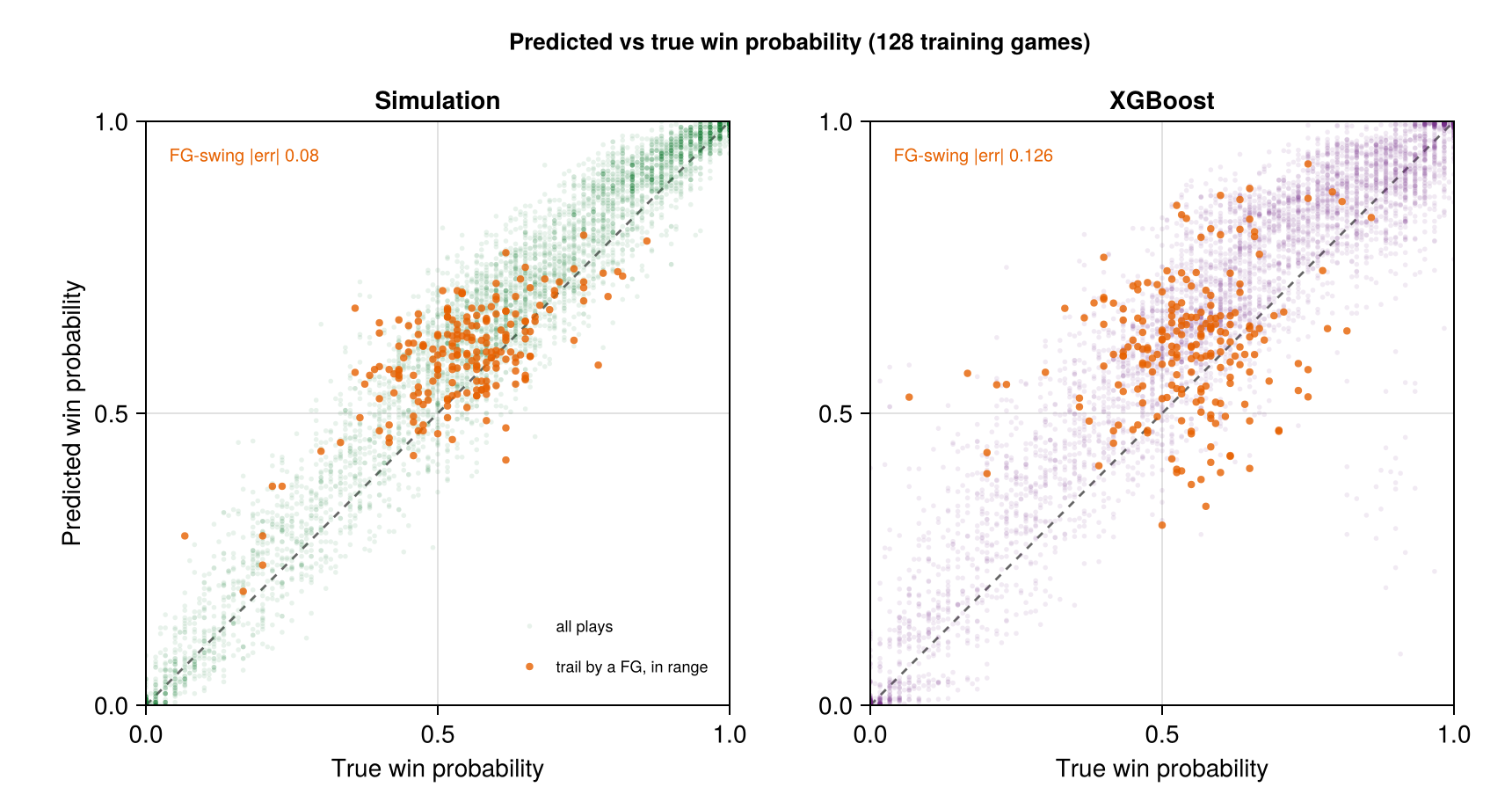
Both models collapse onto the diagonal near 0 and 1 which is exactly why the aggregate Brier looks good. The disagreement lives in the middle and especially on these tight plays. On exactly those plays XGBoost’s mean error climbs to 0.307 while the simulation holds at 0.266: the discriminative model, which has only seen a handful of such moments in 128 games, basically has to guess. The simulation benefits from structure here even though it too has never seen this situation.
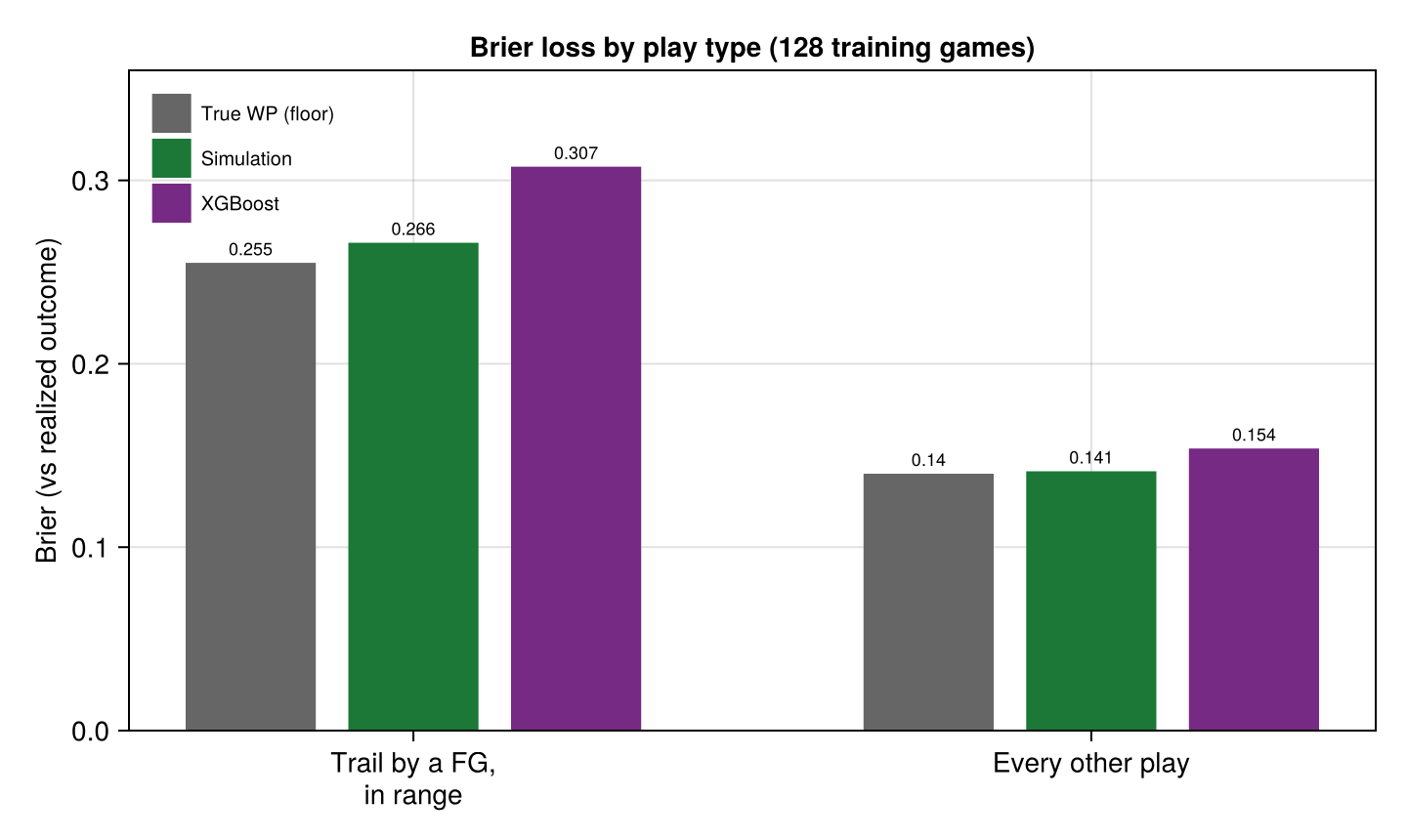
Thus we have a dilemma. For easy states we don’t really need that much data. But for rarer states that often decide games, the very ones we want a win-probability model to get right, we need quite a heck of a lot of data.
This is also the setup’s built-in caveat: on synthetic data the sim is playing on home turf, since the data is drawn from it by construction. To see whether that advantage survives contact with reality, we need real football.
On real data
Here we train on real 2022–2023 play-by-play and score on held-out 2024 plays, with the real nflfastR win-probability model as a reference point. The procedure is identical to the synthetic curve — the only difference is that the true-WP floor is gone (real football doesn’t come with a ground truth) and the training data is genuinely scarce, since the simulation needs play-timestamp coverage that only exists from 2022 on:
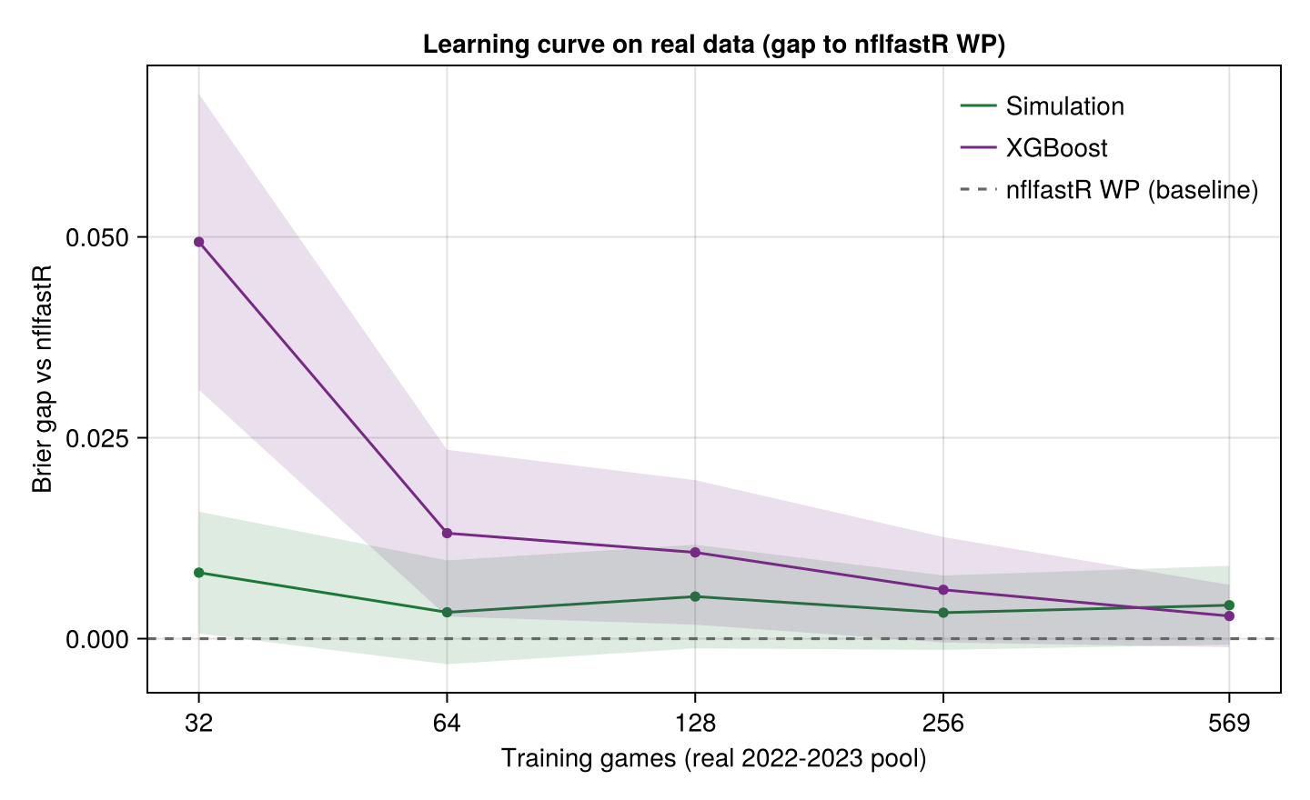
Again we don’t see that much gain in the simulation from the training data. It’s relatively close to the (presumably trained on all available training data) nflFastR model. Our XGBoost replication is much worse though it does catch up by the time we get to a couple seasons.