Win probability models predict the chance a team wins given the current game state. Casual observers underappreciate how difficult this is: there are not many historical football games to provide ground truth, and the game state is complex and dynamic. Those same two problems, scarce outcomes and tangled state, also make the model hard to evaluate. This post is about how we tell whether a win probability is any good, and how our simulation stacks up against the field.
As in training, we use the NFLData.jl package to pull historical play-by-play from the nflverse, and we split it by season into a train set and a held-out test set so that nothing we score on was seen during fitting.
Accounting for correlation
Before discussing any results we need to discuss a complication: auto-correlation.
We make potentially hundreds of predictions per game, but each game gives us a single outcome. Treating those predictions as independent Bernoulli trials is wrong: consecutive predictions are strongly autocorrelated. If team A is 95% likely to win at time \(t-1\), then barring some huge play it is still about 95% likely at time \(t\). Indeed, a model whose win probability bounced around between adjacent plays would be suspect.
For evaluation, the practical consequence is that naive standard errors would be wildly overconfident, treating hundreds of correlated plays as hundreds of independent data points. We fix this with the block jackknife: we estimate the variance of each metric by sequentially dropping entire games from the dataset and re-computing. Deleting whole games removes the within-game correlation that would otherwise leak across the resampling, so the confidence intervals below are honest about how much independent football we actually have (not much!). Every error bar in this post is a block-jackknife interval.
For more discussion go check out Brill, Yurko & Wyner 2024 and note we’ll dig even deeper into this paper in our “How Much Data Does a Win-Probability Model Need?” post.
Metrics
We judge the win probability models three ways.
- Brier score
- The Brier score is a proper scoring rule; you also know it as the mean squared error:
\[ \mathrm{Brier} = \frac{1}{N} \sum_{i=1}^{N} (f_{i} - o_{i})^2 \]
where \(f_i\) is the predicted win probability and \(o_i\) is the outcome (1 for a win, 0 for a loss). Zero is a perfect model; 0.25 is the score you get by predicting 50/50 for everything.
- Log loss
- Log loss is another standard proper scoring rule:
\[ \mathrm{LogLoss} = -\frac{1}{N} \sum_{i=1}^{N} \left[ o_i \log f_i + (1 - o_i) \log (1 - f_i) \right]. \]
It punishes confident-and-wrong far more harshly than Brier does: a prediction of 0.999 that turns out wrong is nearly fatal.
- Calibration
- Both Brier and log loss reward pushing probabilities toward zero and one, as far as the truth allows. Calibration asks a different question: do the estimated probabilities actually behave like probabilities: do they match their long-run frequencies? There’s no number here, rather, we construct a reliability plot. We bucket predictions into bins and compare the nominal probability of each bucket against the observed win rate within it. Points on the diagonal are perfectly calibrated; points below the line mean the model is overconfident, points above mean it is underconfident.
Comparison models
A number is only meaningful next to a baseline. We compare our simulation against the two win probability models the NFL analytics community actually uses.
The nflfastR models
The most widely used public win probability models were both built by Ben Baldwin and Sebastian Carl and ship with nflfastR. Their vanilla model uses XGBoost. They note that they moved from logistic regression to tree-based methods in February 2021 specifically to improve calibration at the end of games, where the interactions between time, field position, and score get particularly gnarly.
The standard folk wisdom in statistics is that you get far more mileage out of better data than out of a better model. The nflfastR folks demonstrate this themselves: their strongest model (nflfastR Vegas) which is the vanilla model plus a single extra feature: the Vegas spread at kickoff. That one feature buys a large edge early in games, where the pregame market knows far more than the box score does. As we will see, the gap shrinks as the game goes on and the in-game situation takes over.
There is one slight problem: I have no idea what data they trained on. That creates two headaches for a clean comparison:
- If their training set overlaps our test seasons, we would overstate their performance: they would be scored partly on games they already saw.
- We cannot equalize the amount of training data. We want any difference to be a property of the model, not just the fact that nflfastR sees far more football.
So alongside the published models we fit our own retrain of the nflfastR XGBoost specification on exactly the seasons our simulation sees.
That “nflfastR (retrain)” model controls for the data advantage.
It appears in every plot below next to the published nflfastR model.
Win probability results
Here is the headline: overall Brier and log loss across the held-out test seasons, with block-jackknife 95% intervals. Lower is better.
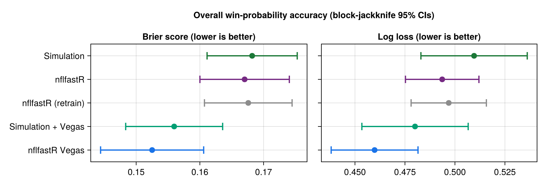
And we see that we have basically overlapping performance! We have two clear regimes: obviously the Vegas information is superior, but within those two groups we can’t clearly distinguish which is better.
Looking then at calibration:
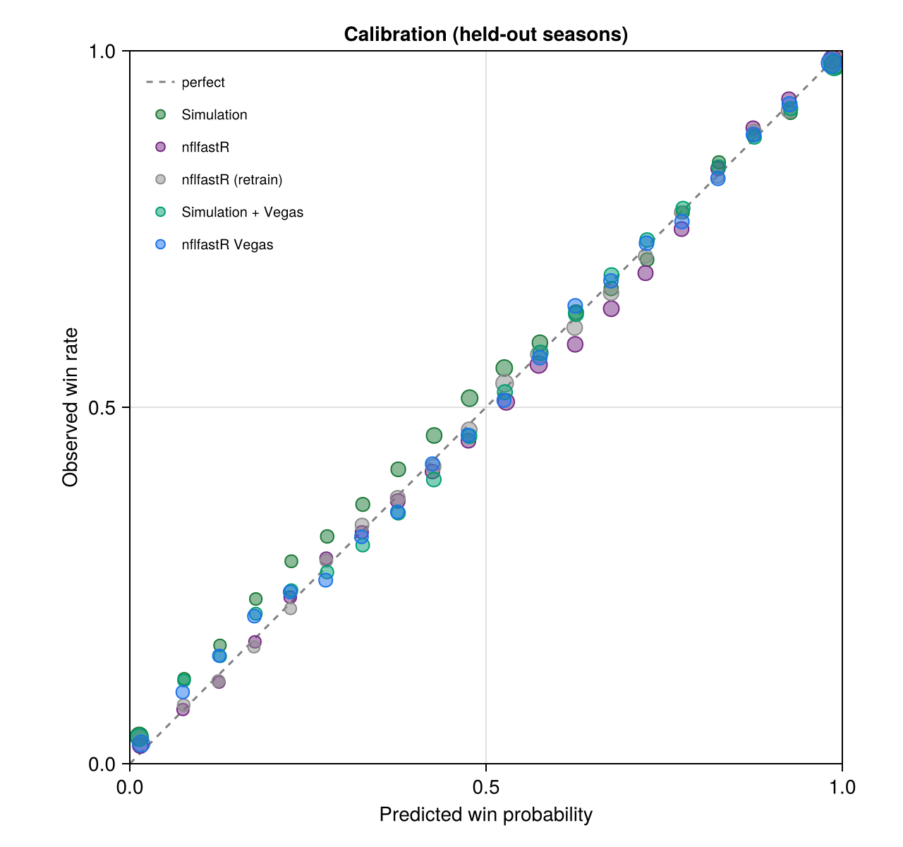
The NFLFastR models are along the diagonal nicely: the simulation is a bit more off especially in the lower half of the plot: it’s a little too overconfident (likely missing some comeback features).
Slicing by time
As a game goes on, the outcome gets more and more certain: for a blowout, every model converges to nearly 100% and there is no skill to demonstrate. The tight games late are where a better model can actually separate. So we slice the Brier score by how much game time remains.
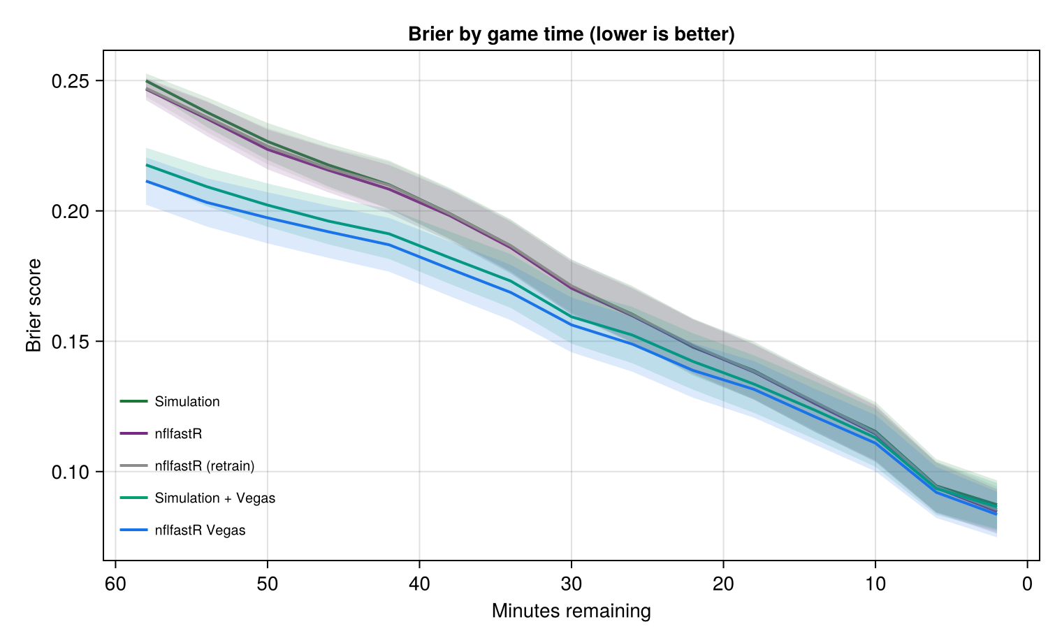
This indicates the nature of the Vegas bonus: it’s a huge gap at the start of the game and then converges with the rest of the field in the endgame as there the structure of the game dominates and everything looks more or less the same.
Everywhere, that is, except for one special situation this plot leaves out: overtime!
In overtime the simulators post the best Brier (0.21 for Simulation + Vegas, 0.21 for the team-agnostic simulation), while the two published nflfastR models are the worst of the field (0.23 apiece).
Overtime is rare, so regression models trained on whole-game data have barely seen it; a simulator that simply keeps playing sudden death out doesn’t care that it’s rare: it’s still just play after play.
Expected points
Win probability is not the only outcome the simulation can give us. Every rollout plays the rest of the game out to the end, so the same machinery that tells us who wins also tells us how the scoring unfolds. Thus we can also estimate expected points (EP).
Same as before: we’ll compare against nflfastR’s published model and we don’t know what data it’s trained on. So we also train our own copy of nflfastR’s EP model to the same specification (a seven-class multinomial with their hyperparameters) on the same seasons our simulation sees.
But first we need to figure out what exactly we mean by “expected points”.
Two definitions
There are (at least) two reasonable answers.
The intuitive one is drive expected points: from the current play, how many net points does the team with the ball go on to score through the end of this possession? A touchdown is worth 7, a field goal 3, a punt or turnover 0, and the only way to go negative is a safety at -2.
The standard one, used by nflfastR and essentially everyone else, is next-score expected points: the signed value of the next score by either team before the half ends. If you punt and your opponent drives down to score, that next score counts against you. So this EP can be sharply negative when you are pinned deep in your own end.
Next-score EP feels a little unnatural: why should the value of my 1st-and-10 be dragged down by a touchdown the other team scores three possessions from now? It goes back to a very old (1971!) paper “Operations Research on Football”, which coded a season of plays and computed, for each spot on the field, the average value of the next score. Yurko, Ventura, and Horowitz formalized the modern version in nflWAR (2019) as a multinomial over the seven possible next-scoring events (your touchdown / field goal / safety, the same three for your opponent, or no score) within the current half. This is useful because it helps you quantify the effect of field position: you should get penalized for giving up position to your opponent above and beyond just the penalty for not scoring yourself.
Results
We’ll compare RMSEs now:
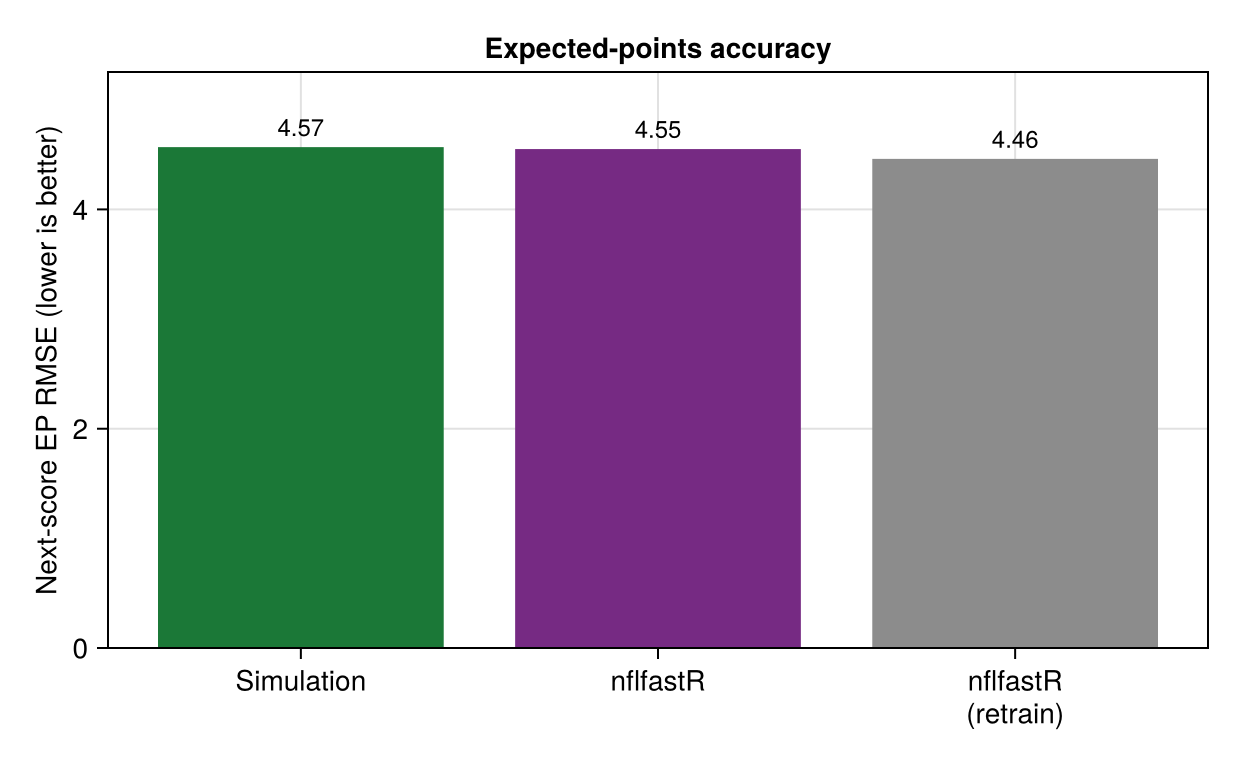
And we get the same story as before: we’re basically statistically identical with the discriminative model (though we could probably benefit from more data).
Conclusion
Thus it seems like we have a decent enough model: we’re statistically similar to a prominent open source model and we get a lot more interpretability out of it. We’ll see though that we can use this for far more interesting things than prediction in our next post: How much data does it need?