As we discussed in the previous post, the Bradley Terry model is a pairwise comparison model where each entity has strength \(\gamma_{i}\) and the probability of victory for entity \(a\) over entity \(b\) is
\[ \Pi_{a,b} = \text{logistic}(\gamma_{a} - \gamma_{b}) \]
which is just a fancy logistic regression.
You can almost immediately see the problem when applying this to rock-paper-scissors. Rock beats scissors is fine: \(\gamma_{\text{rock}} > \gamma_{\text{scissors}}\). And scissors beats paper is again fine: \(\gamma_{\text{scissors}} > \gamma_{\text{paper}}\). But for paper to beat rock we need \(\gamma_{\text{paper}} > \gamma_{\text{rock}}\) and due to the inherent linearity of numbers that simply isn’t possible. Hence we need to do something else.
Extending to Non-Transitivity
So what can we do instead1? There is a natural clustering suggested by the rock-paper-scissors example so let’s use it. We augment each entity with a latent cluster \(Z_{i}\) and a matrix \(A_{c_{1}, c_{2}}\) of the advantage an entity of cluster \(c_{1}\) would have over an entity of cluster \(c_{2}\). Then the probability becomes
\[ \Pi_{a,b} = \text{logistic}(\gamma_{a} - \gamma_{b} + A_{Z_{a}, Z_{b}}) \]
which hopefully starts to capture our non-transitivity!
Fitting this is a bit of a mess; but fortunately we can express this as a Bayesian model and turn the computational crank with MCMC.
Simulation
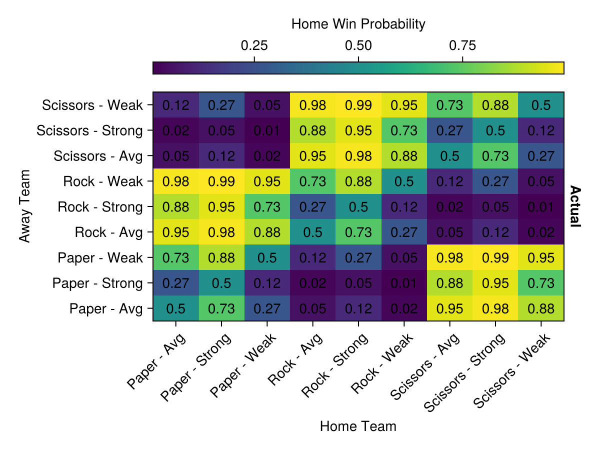
So let’s now try it on a simulated rock-paper-scissors-like data. We’ll have three competitors in each class with low, medium, and high skills and simulate some games.
You can clearly see the rock-paper-scissors pattern in the true probability graph. There’s clearly major blocks where group dynamics dominate with some slight variation due to intrinsic skill. But the weakest rock player is still favored against the strongest scissors player.
Vanilla Bradley Terry
Before we start looking at the cluster approaches we can start by showing the shortcomings of the vanilla Bradley Terry model on this data. The Turing code is quite straightforward:
using Distributions
using Turing

@model function BradleyTerry(match_data)
    n_entities = match_data.n_entities

    # Individual strengths
    β ~ filldist(Normal(0, 1), n_entities)

    # Likelihood
    for ii in eachindex(match_data.lo_wins)
        lo = match_data.lo_ids[ii]
        hi = match_data.hi_ids[ii]
        logit_p = β[lo] - β[hi]
        match_data.lo_wins[ii] ~ Binomial(match_data.matches[ii], logistic(logit_p))
    end

    # Generated quantities
    win_probabilities = [logistic(β[ii] - β[jj]) for ii = 1:n_entities, jj = 1:n_entities]
    return win_probabilities
end
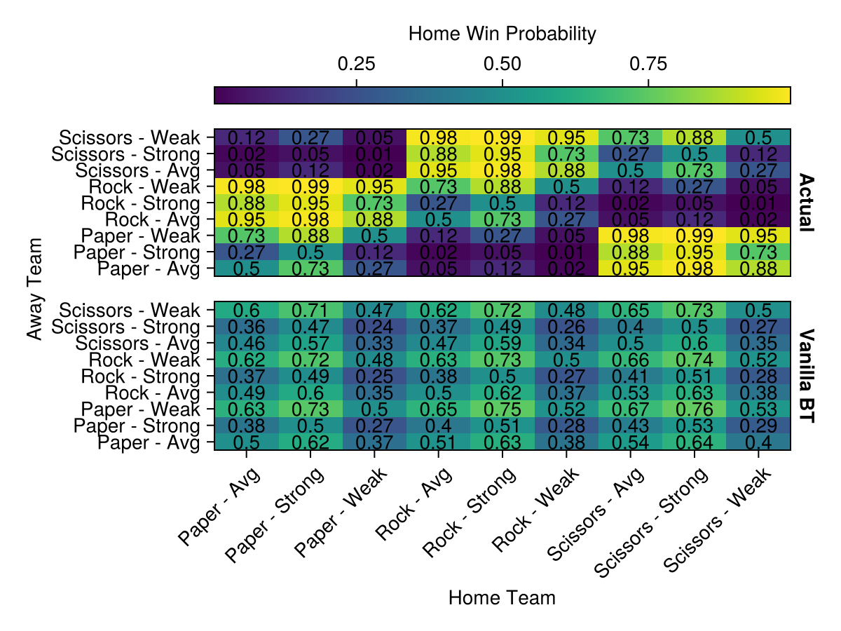
Because it can’t represent nontransitivity it fails pretty hard. It ends up smearing everyone’s ability level since seemingly weak in-cluster competitors are demolishing strong outside-cluster competitors and our model has no idea how to account for that.
Clustered Bradley Terry
Now we introduce our clustering approach. The beauty of a PPL like Turing is that we don’t have to modify our code too much. There’s a little bit of messing around we have to do to enforce symmetry in the cluster advantages (\(A_{i,j} = -A_{j,i}\)).
function get_cluster_effect(ut::AbstractVector{T}, idx1, idx2) where {T}
    idx1 == idx2 && return zero(T)
    if idx1 < idx2
        idx = idx1 + div((idx2 - 1) * (idx2 - 2), 2)
        return ut[idx]
    else
        idx = idx2 + div((idx1 - 1) * (idx1 - 2), 2)
        return -ut[idx]
    end
end

@model function ClusteredBradleyTerry(match_data, max_clusters = 3)
    n_entities = match_data.n_entities

    # Individual strengths
    β ~ filldist(Normal(0, 1), n_entities)

    # Cluster effects
    n_cluster_pairs = div(max_clusters * (max_clusters - 1), 2)
    cluster_ut ~ filldist(Normal(0, 1), n_cluster_pairs)

    cluster = [1, 1, 1, 2, 2, 2, 3, 3, 3] # fixed (for now)

    # Likelihood
    for ii in eachindex(match_data.lo_wins)
        lo = match_data.lo_ids[ii]
        hi = match_data.hi_ids[ii]
        logit_p = β[lo] - β[hi] + get_cluster_effect(cluster_ut, cluster[lo], cluster[hi])
        match_data.lo_wins[ii] ~ Binomial(match_data.matches[ii], logistic(logit_p))
    end

    # Generated Quantities
    win_probabilities = [
        logistic(β[ii] - β[jj] + get_cluster_effect(cluster_ut, cluster[ii], cluster[jj])) for ii = 1:n_entities, jj = 1:n_entities
    ]
    return win_probabilities
end
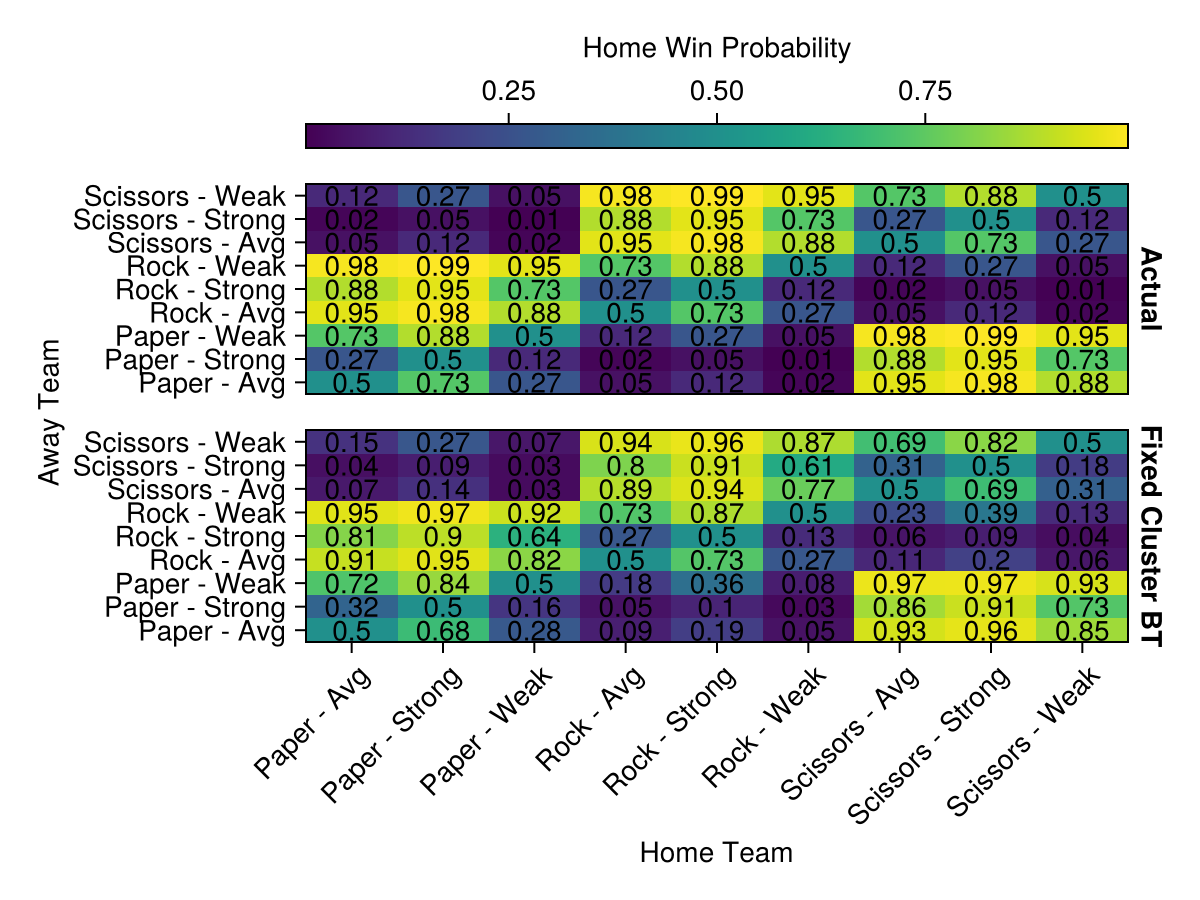
We find that this works amazingly! We learn the appropriate rock-paper-scissors stucture as is apparent in the figure. The only unfortunate bit is that we had to specify the clusters themselves. Your natural question might be whether we can actually learn the clusters themselves?
Dirichlet Process Bradley Terry
Now let’s work with our model introducing a non-parametric clustering using Dirichlet Processes. This is a way to put a prior on clusters where we have a potentially infinite number of clusters. We, of course, don’t have infinite data so we end up with a finite number of clusters. Working with infinite dimensional paramters is tricky so we also truncate it to a finite dimension for practicality (but still much larger than any reasonable number of clusters).
The one knob worth thinking about is the concentration parameter \(\alpha\) in the stick-breaking prior: it sets how eagerly the process spawns new clusters. The expected number of occupied clusters grows roughly like \(\alpha \log(1 + n/\alpha)\), so a large \(\alpha\) pushes towards many small clusters. With only nine entities and three “true” groups we want a fairly parsimonious prior, so we set \(\alpha = 1\).
using Turing.RandomMeasures

@model function BradleyTerryDP(match_data, max_clusters = 9, α = 1.0)
    n_entities = match_data.n_entities

    # Individual strengths
    β ~ filldist(Normal(0, 1), n_entities)

    # Cluster assignments
    v ~ filldist(Beta(1, α), max_clusters - 1)
    normalized_weights = Turing.RandomMeasures.stickbreak(v)
    cluster ~ filldist(Distributions.Categorical(normalized_weights), n_entities)

    # Cluster effects
    n_cluster_pairs = div(max_clusters * (max_clusters - 1), 2)
    cluster_ut ~ filldist(Normal(0, 1), n_cluster_pairs)

    # Likelihood
    for ii in eachindex(match_data.lo_wins)
        lo = match_data.lo_ids[ii]
        hi = match_data.hi_ids[ii]
        logit_p = β[lo] - β[hi] + get_cluster_effect(cluster_ut, cluster[lo], cluster[hi])
        match_data.lo_wins[ii] ~ Binomial(match_data.matches[ii], logistic(logit_p))
    end

    # Generated Quantities
    win_probabilities = [
        logistic(β[ii] - β[jj] + get_cluster_effect(cluster_ut, cluster[ii], cluster[jj])) for ii = 1:n_entities, jj = 1:n_entities
    ]
    return win_probabilities
end
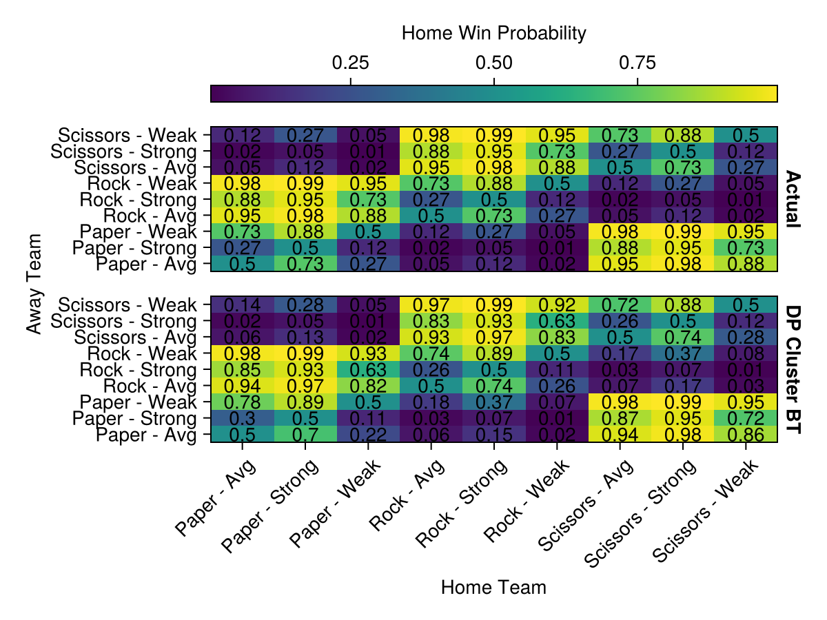
And we see that we recover the structure just as well as before! And we didn’t have to specify or even really hint at any potential structure: the model found the structure itself.
To verify we can indeed look at the clustering stucture itself (aside from the implicit confirmation from the win probability heatmap). This gets tricky due to label switching: we can totally swap the labels for the rock cluster the paper cluster and with some swaps of the other parameters there’ll be no change in our likelihood or prior probabilities. You can see this particularly strongly when you fit multiple chains as each permutation is roughly equally likely when initializing.
The best way to work with these sorts of parameters is to instead transform them into quantities which are invariant to permutations. In particular we might consider the coclustering matrix where each entry (i, j) counts the proportion of samples for which entity \(i\) is in the same cluster as entity \(j\). This will reveal the clustering behavior unaffected by label switches.
function coclustering_matrix(chain, n_entities)
    # samples × entities matrix of integer cluster labels
    labels = Int.(param_samples(chain, :cluster))
    n_samples = size(labels, 1)
    co = zeros(n_entities, n_entities)
    for s = 1:n_samples, i = 1:n_entities, j = 1:n_entities
        co[i, j] += (labels[s, i] == labels[s, j]) / n_samples
    end
    return co
end
Ordering the entities by their most frequent cluster makes the block-diagonal rock-paper-scissors structure pop right out.
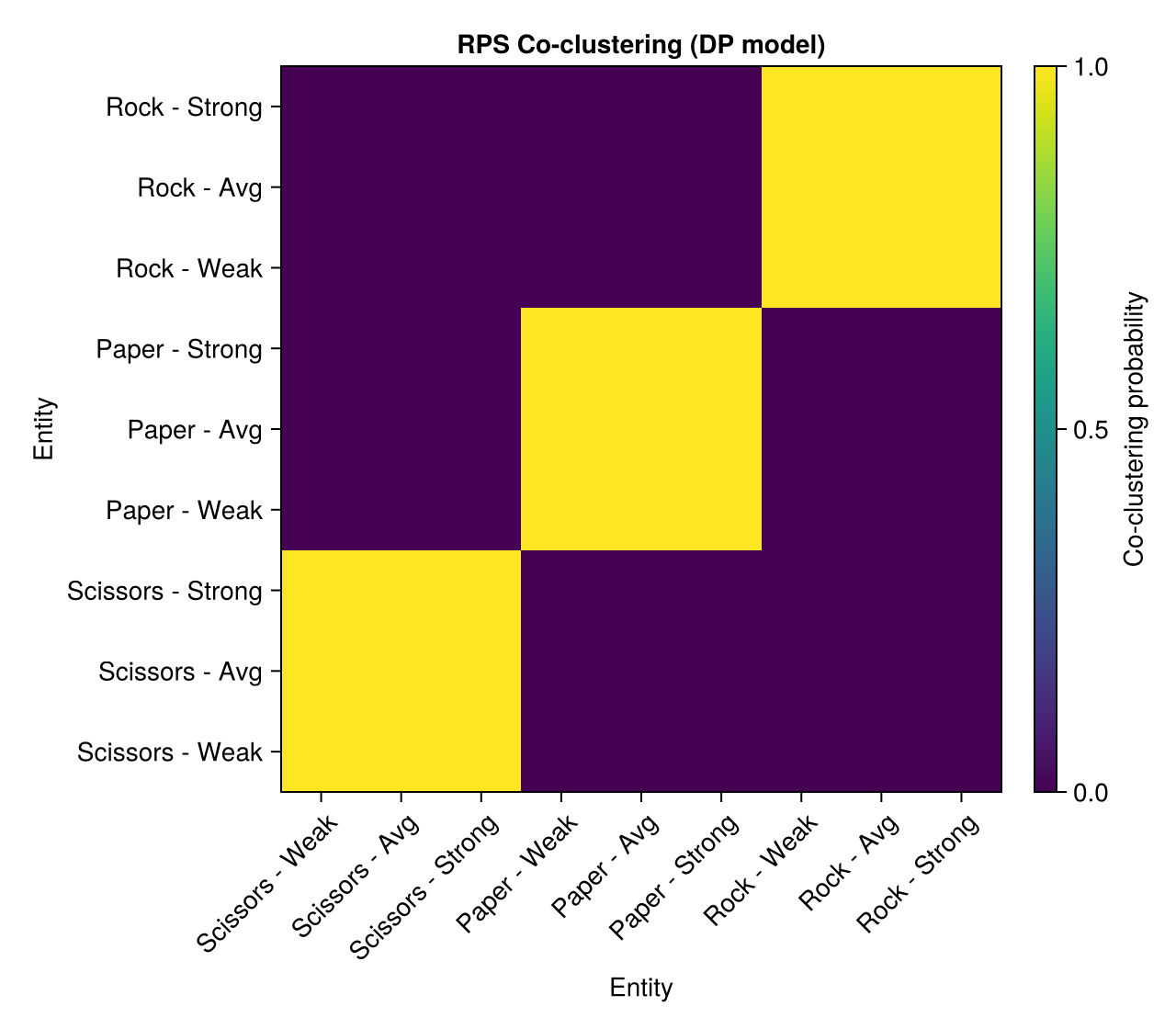
The three rock-paper-scissors blocks light up clearly: entities sharing a base type are coclustered with high probability regardless of their individual skill, and almost never coclustered across base types.
Getting here was fiddly, though. Sampling discrete cluster assignments is genuinely hard: we had to greatly increase our iterations and burn-in and on roughly a third of random seeds we still got stuck reporucing vanilla Bradley Terry. And it gets worse the large the number of cluster assigments we need to work through. The large discrete space is hard to explore: to properly scale this we need something smoother.
A Differentiable Relaxation: Soft Clustering
The textbook fix for a discrete latent variable is to marginalize it out, and here that looks like a trap. Each entity’s cluster is shared across all of its matches, so an honest marginalization sums over all \(K^{n}\) joint assignments of every entity to a cluster — hopeless beyond toy data.
So rather than force a hard assignment, let’s relax it. Give each entity a soft membership vector \(p_{i}\) and take the advantage to be the expected advantage under those memberships:
\[ A_{i,j} = p_{i}’ A p_{j} \]
When membership concentrates on a single cluster this recovers the hard assignment exactly, but everything is now continuous. This also gets us the benefit of being able to use reverse-mode AD which works nicer. We keep the Dirichlet-process flavour by centering each entity’s membership logits on the shared stick-breaking log-weights: clusters stay empty unless the data actively pushes an entity into them, so the model still discovers how many groups it needs.
using ReverseDiff, Memoization # now we can use reverse-mode
using StatsFuns: softmax
using LinearAlgebra: dot

@model function SoftClusterBradleyTerry(match_data, max_clusters = 9)
    n_entities = match_data.n_entities

    # Individual strengths
    β ~ filldist(Normal(0, 1), n_entities)

    # Cluster weights (stick-breaking, exactly as in the discrete model)
    α = 1.0
    v ~ filldist(Beta(1, α), max_clusters - 1)
    log_weights = log.(Turing.RandomMeasures.stickbreak(v))

    # Cluster effects
    n_cluster_pairs = div(max_clusters * (max_clusters - 1), 2)
    cluster_ut ~ filldist(Normal(0, 1), n_cluster_pairs)
    A = [get_cluster_effect(cluster_ut, k, m) for k = 1:max_clusters, m = 1:max_clusters]

    # Soft memberships: per-entity logit offsets from the shared weights
    Z ~ filldist(Normal(0, 2), n_entities, max_clusters)

    # Likelihood
    for ii in eachindex(match_data.lo_wins)
        lo = match_data.lo_ids[ii]
        hi = match_data.hi_ids[ii]
        p_lo = softmax(log_weights .+ Z[lo, :])
        p_hi = softmax(log_weights .+ Z[hi, :])
        logit_p = β[lo] - β[hi] + dot(p_lo, A * p_hi)
        match_data.lo_wins[ii] ~ Binomial(match_data.matches[ii], logistic(logit_p))
    end

    # The generated quantities don't play nicely with AD so we drop it

    return nothing
end
We reconstruct win probabilities from the samples in the same expected way: averaging \(p_{i}^{\top} A\, p_{j}\) over the posterior. We do this outside of the generator since we’re looking to be performant and making these inside the PPL just adds to the burden on the autodiff.
function soft_win_probabilities(chain, match_data, max_clusters = 9)
    β_samples = param_samples(chain, :β)
    v_samples = param_samples(chain, :v)
    ut_samples = param_samples(chain, :cluster_ut)
    Z_samples = vec(chain[:Z])

    n_samples, _ = size(β_samples)
    n_entities = match_data.n_entities
    win_probs = zeros(n_entities, n_entities)

    for s = 1:n_samples
        β = β_samples[s, :]
        log_weights = log.(Turing.RandomMeasures.stickbreak(v_samples[s, :]))
        A = [
            get_cluster_effect(ut_samples[s, :], k, m) for
            k = 1:max_clusters, m = 1:max_clusters
        ]
        memberships = [softmax(log_weights .+ Z_samples[s][i, :]) for i = 1:n_entities]

        for ii = 1:n_entities, jj = 1:n_entities
            win_probs[ii, jj] +=
                logistic(β[ii] - β[jj] + dot(memberships[ii], A * memberships[jj])) /
                n_samples
        end
    end

    return win_probs
end
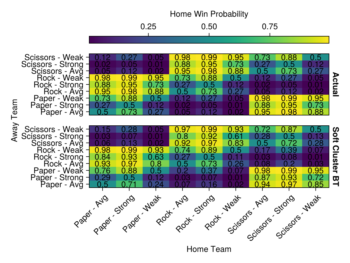
When we look at the results we again recapture the rock-paper-scissors structure as before. This time much more quickly and reliably: neither finicky nor slow. Comparing the wall-clock fit times (each including one-time compilation) shows just how lopsided it is on this small example:
| Method | Fit time (s) |
|---|---|
| DP (discrete particle Gibbs) | 429.0 |
| Soft clustering (reverse-mode NUTS) | 55.6 |
The soft model is the clear winner: it recovers the same structure, runs the better part of an order of magnitude faster, and lands in the right basin reliably rather than playing the seed-roulette of the discrete sampler. As a bonus the soft memberships are themselves more informative than hard labels and the co-clustering matrix falls straight out of them as \(E[p_{i}‘p_{j}]\):
function soft_cluster_recovery(chain, match_data, max_clusters = 9)
    v_samples = param_samples(chain, :v)
    Z_samples = vec(chain[:Z])
    n_samples = length(Z_samples)
    n_entities = match_data.n_entities

    cluster_probs = zeros(n_entities, max_clusters)
    coclustering = zeros(n_entities, n_entities)

    for s = 1:n_samples
        log_weights = log.(Turing.RandomMeasures.stickbreak(v_samples[s, :]))
        memberships =
            reduce(vcat, [softmax(log_weights .+ Z_samples[s][i, :])' for i = 1:n_entities])
        cluster_probs .+= memberships ./ n_samples
        coclustering .+= (memberships * memberships') ./ n_samples
    end

    return cluster_probs, coclustering
end
Application: Pokemon!
For a “real” example we can use the Weedle’s cave data set from Kaggle which captures battle outcomes between different Pokemon. Now those of you born in the 90s will know2 that Pokemon have types and these types exhibit rock-paper-scissors dynamics: electric is super effective against water which is super effective against fire and so on. In addition Pokemon have the own individual stats and thus a strong Pokemon might still be favored against a opponent of a type it’s weak against. This seems like a natural fit for our model!
We start by fitting the same fixed clustered model as before just at a much larger scale now. This model still runs relatively quickly and works quite well:
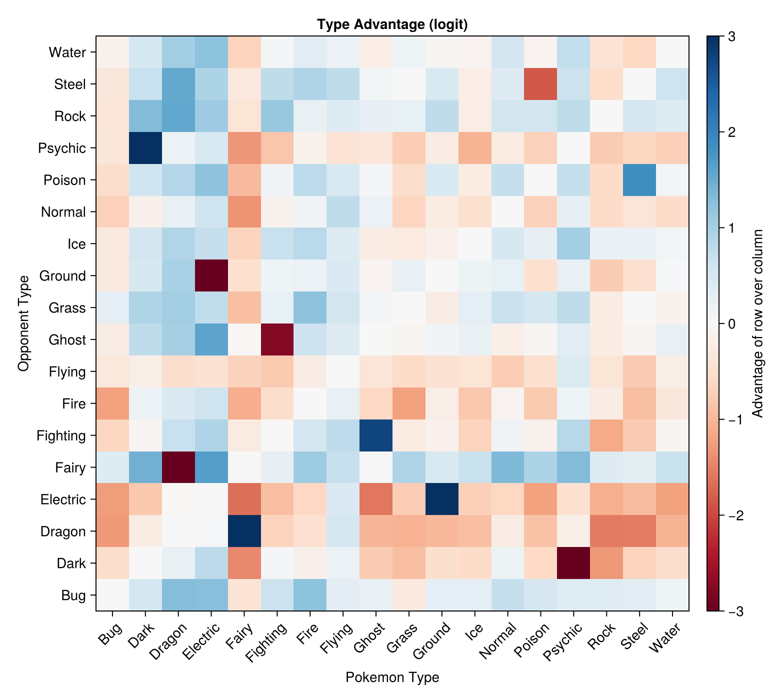
Evaluating solely on reconstructing the type advantage is a bad idea so we’ll use some hold-out predictions. We should see some improvement by incorporating our type advantages on top of individual skill. This is indeed what we see but the gains are relatively marginal. This dataset is dominated by individual skill which greatly outweigh the class advantages.
| Model | Test log-loss | Test accuracy |
|---|---|---|
| Vanilla BT | 0.35 | 0.885 |
| Type-aware BT (known types) | 0.332 | 0.891 |
| Soft-cluster BT (learned) | 0.353 | 0.883 |
The interesting case is the last row. The fixed model when handed the true types, squeezes out a small win. But when we ask the soft-cluster model to discover the groups from match outcomes alone, it can’t find the type structure: it does slightly worse than vanilla Bradley Terry. Poking at the fit shows why. The handful of clusters it does settle on track raw skill rather than type: their advantage matrix comes out essentially transitive (a stronger group beating a middling group beating a weaker one), and cluster membership has basically nothing to do with a Pokemon’s actual type. The model is just re-encoding the individual strengths \(\gamma\) it already has.
This makes sense. Type advantages here are both small and badly confounded with individual skill as a strong fire Pokemon beats most water Pokemon not because of it’s advantaged (the opposite actually) but because it is simply strong. Recovering a non-transitive cycle means seeing the same entities both beat and lose to each other depending on the matchup, and once you condition on skill there just isn’t enough of that left in the data. The rock-paper-scissors signal that jumped straight out of the toy data is, in real Pokemon battles, mostly drowned out by raw stats. We’ll look deeper into this in the next post!
-
This is perhaps equivalent to this paper although I can’t quite tell as it’s confusingly written. They additionally put a Dirichlet Process on the \(\gamma\) terms which doesn’t make a ton of sense to me although they justify it by pointing that with match data certain entities are just statistically indistinguishable. ↩︎
-
I know this only second-hand as my parents thought books were better than GameBoys: look at the ruin they brought upon me ↩︎