It turns out I have at least a trilogy about Bradley Terry models in me! Let’s revisit the Pokemon data that we discussed last time. One of the salient features of Pokemon is that they grow: they increase their stats, get new abilities, and sometimes even evolve into a new species. Very cool and fun; but it wrecks our models!
Quick recap: the Bradley Terry model gives entities a latent strength \(\gamma_{i}\) and the probability that entity \(a\) beats entity \(b\) is
\[ \Pi_{a,b} = \sigma(\gamma_{a} - \gamma_{b}) \]
The issue is the assumption of a fixed strength. Consider the state right before and right after evolving. Say we were evenly matched before so \(\gamma_{a} = \gamma_{b}\). But surely we’re more likely to win now that we’ve increased our stats so \(\gamma_{a} > \gamma_{b}\). 1
There are two-ish ways to accommodate this within vanilla-ish BT:
-
The first is to just treat the evolved Pokemon as a completely new entity. This loses a lot of data but it works. The only issue is that Pokemon gain XP for every battle. By the time you’ve collected enough data at the new level they’re ready to level-up again and your data is useless again.
-
The more general approach is to try to explicitly model the trajectory of abilities. Essentially you make a hidden Markov model where \(\gamma\) evolves over time and matches are observations. We’re actually in a relatively nice state since we know exactly when the transitions happened and we can make the assumption that evolutions monotonically increase \(\gamma\) but still it’s a lot of assumptions and not a lot of data to fit them with.
So I’d like to instead investigate an alternate approach: dropping the ability to measure any individual Pokemon’s skills. Instead we take each Pokemon’s baseline statistics and use them to directly predict strength. In particular we model
\[ \gamma_{i} = NN(x_{i}) \]
where \(x_{i}\) is the stat vector and \(NN\) is a small feed-forward network. This lets us generalize immediately to any stat combination we’ve never seen before including newly evolved Pokemon!
Data and competing models
We’ll continue to use the Weedle’s Cave dataset from Kaggle, which gives us the base stats for 800 Pokemon and 50k battle outcomes.
Each Pokemon’s feature vector consists of its six base stats (normalized to [0,1]) plus a one-hot encoding of its primary type (there are secondary types but we’ll ignore that for now).
To compare our model we need some reference points. The crudest is a speed heuristic: simply predict that the faster Pokemon wins. Speed turns out to be so correlated with the outcome that this is a deceptively strong baseline: strong enough, as we’ll see, to embarrass our neural network.
A more conventional benchmark is vanilla Bradley Terry: the model from the previous posts that gives each individual Pokemon its own latent strength \(\gamma_{i}\) with no features at all. On familiar Pokemon it is a reasonable baseline; its weakness is that it has nothing to say about a Pokemon it has never seen. For consistency with our next model we’ll write this in Flux instead of the Turing we’ve used before.
struct VanillaBT
    γ::Vector{Float32}
end
Flux.@layer VanillaBT
bt_predict(m::VanillaBT, ia, ib) = σ.(m.γ[ia] .- m.γ[ib])

function train_vanilla_bt!(m, ia, ib, y; epochs = 80, batchsize = 256, lr = 1e-2)
    opt_state = Flux.setup(Adam(lr), m)
    loader = Flux.DataLoader((ia, ib, y), batchsize = batchsize, shuffle = true)
    for _ = 1:epochs
        for (ia_b, ib_b, y_b) in loader
            grads = Flux.gradient(m) do mdl
                loglike(bt_predict(mdl, ia_b, ib_b), y_b)
            end
            Flux.update!(opt_state, m, grads[1])
        end
    end
end
Neural Bradley Terry
With the data and competing models in hand, let’s build the neural BT model. As mentioned before the strength network maps a feature vector to a scalar:
\[ \gamma_{i} = NN(x_{i}) \]
and the match prediction is exactly the standard Bradley Terry formula:
\[ \Pi_{a,b} = \sigma(\gamma_{a} - \gamma_{b}) = \sigma(NN(x_{a}) - NN(x_{b})) \]
Note the important symmetry: by construction \(\Pi_{a,b} + \Pi_{b,a} = 1\), because swapping \(a\) and \(b\) negates the argument of \(\sigma\).
This is exactly the neural Bradley Terry formulation from the literature: push each item’s feature vector through a shared network to get a scalar score and then compare scores. In fact the Weedle’s Cave data is exactly the same dataset they used (and how I became aware of both this approach and dataset).
We train by maximising the log-likelihood just as we would with vanilla BT just with the more complicated neural network
function loglike(p, y)
    -mean(@. y * log(p + 1e-7) + (1.0 - y) * log(1.0 - p + 1e-7))
end

function train_strength_model!(
    net,
    Xa_tr,
    Xb_tr,
    Y_tr;
    epochs = 80,
    batchsize = 256,
    lr = 1e-3,
)
    opt_state = Flux.setup(Adam(lr), net)
    loader = Flux.DataLoader((Xa_tr, Xb_tr, Y_tr), batchsize = batchsize, shuffle = true)
    for _ = 1:epochs
        for (xa_b, xb_b, y_b) in loader
            grads = Flux.gradient(net) do m
                p = σ.(vec(m(xa_b)) .- vec(m(xb_b)))
                loglike(p, y_b)
            end
            Flux.update!(opt_state, net, grads[1])
        end
    end
end

strength_net = Chain(Dense(n_features, 32, relu), Dense(32, 16, relu), Dense(16, 1))
train_strength_model!(strength_net, Xa_train, Xb_train, Y_train)
Results
We split our data into train and validation sets, splitting 80/20 by battle. We calculate the accuracy and find a humbling result.
| Model | Val Accuracy |
|---|---|
| Speed heuristic | 0.9421 |
| Vanilla BT | 0.8851 |
| Neural BT (literature) | 0.8899 |
The plain neural network barely edges out vanilla BT and loses outright to “just look at who’s faster.” All those base stats and a one-hot type, fed through a neural network, and we can’t beat a one-liner. The problem is that strength is fundamentally additive in this model: it collapses each Pokemon to a single scalar and can’t represent the fact that being fast is not so important as being faster. We’ll need to address this to improve our performance.
But first let’s see what the strength network actually learned. If we plot \(NN(x_{i})\) against total base stats for every Pokemon, we can check that the model has found a sensible strength ordering.
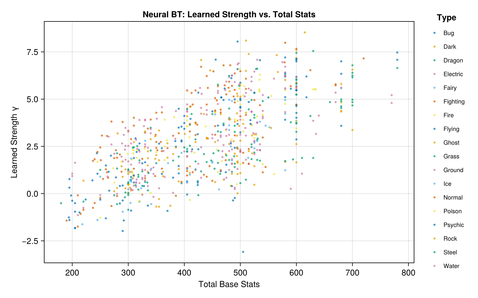
Figure 1: Plot of neural network strengths (gamma_{i}) against total base stats: we see a reasonable correlation: higher stats → higher strength as expected
The strength is roughly monotone in total stats as expected but with substantial scatter along the trend line. There’s a notable outlier with the weakest Pokemon by learned strength still having base stats of 500+. That would be Shuckle: its 505 stat total is almost entirely Defense and Sp. Def (230 each) with a Speed of 5. Not surprisingly Shuckle lost every single one of its 135 battles.
Adding Interactions
So the base model treats every matchup additively: Pokemon \(a\) beats \(b\) iff \(\gamma_{a} > \gamma_{b}\). But as we remember from the previous post, Pokemon types create a rock-paper-scissors structure that can’t be captured this way. But more importantly as we’ve seen before speed is super important but mostly in relation to the speed of the other Pokemon!
We’d like to add an interaction term that captures these. We could just do the fixed clustering as before but that would be giving up the generalization benefit of the neural network and makes it hard to model the speed interaction. So instead let’s add another network:
\[ \Pi_{a,b} = \sigma\!\bigl(NN(x_{a}) - NN(x_{b}) + SASNN(x_{a}, x_{b})\bigr) \]
where \(SASNN\) must satisfy the antisymmetric constraint \(SASNN(x_{a}, x_{b}) = -SASNN(x_{b}, x_{a})\). We need this constraint to continue to guarantee \(\Pi_{a,b} + \Pi_{b,a} = 1\).
Constructing such a network is easy and a standard trick in ranking models: take any standard network \(f\) and define
\[ SASNN(x_{a}, x_{b}) = f(x_{a}, x_{b}) - f(x_{b}, x_{a}) \]
Swapping \(a\) and \(b\) negates itself by construction! Of course there’s some identifiability issues but this is deep learning so we won’t worry too much about it.
struct SASNN
    f::Chain
end
Flux.@layer SASNN

function (m::SASNN)(xa::AbstractMatrix, xb::AbstractMatrix)
    vec(m.f(vcat(xa, xb))) .- vec(m.f(vcat(xb, xa)))
end
function (m::SASNN)(xa::AbstractVector, xb::AbstractVector)
    only(m.f(vcat(xa, xb))) - only(m.f(vcat(xb, xa)))
end

struct NeuralBT
    strength::Chain
    ssnn::SASNN
end
Flux.@layer NeuralBT

function predict(m::NeuralBT, xa, xb)
    γ_diff = vec(m.strength(xa)) .- vec(m.strength(xb))
    return σ.(γ_diff .+ m.ssnn(xa, xb))
end

function full_loss(m::NeuralBT, xa, xb, y)
    return loglike(predict(m, xa, xb), y)
end

ssnn_inner = Chain(Dense(2 * n_features, 32, relu), Dense(32, 16, relu), Dense(16, 1))
full_model = NeuralBT(
    Chain(Dense(n_features, 32, relu), Dense(32, 16, relu), Dense(16, 1)),
    SASNN(ssnn_inner),
)

function train_joint_model!(
    model,
    Xa_tr,
    Xb_tr,
    Y_tr;
    epochs = 80,
    batchsize = 256,
    lr = 1e-3,
)
    opt_state = Flux.setup(Adam(lr), model)
    loader = Flux.DataLoader((Xa_tr, Xb_tr, Y_tr), batchsize = batchsize, shuffle = true)
    for _ = 1:epochs
        for (xa_b, xb_b, y_b) in loader
            grads = Flux.gradient(model) do m
                loglike(predict(m, xa_b, xb_b), y_b)
            end
            Flux.update!(opt_state, model, grads[1])
        end
    end
end

train_joint_model!(full_model, Xa_train, Xb_train, Y_train)
We check performance again and thankfully find that the interaction term finally helps us clear the speed heuristic.
| Model | Val Accuracy |
|---|---|
| Neural BT (literature) | 0.8899 |
| Speed heuristic | 0.9421 |
| Neural BT + SASNN | 0.9534 |
Generalizing to Unseen Pokemon
So far every model has seen every Pokemon during training: the held-out battles just pair up familiar fighters in new combinations. But the whole motivation for neural BT was generalizing to entities we’ve never seen: a freshly evolved Pokemon with a stat line that never appeared in training.
To stress-test this we change the split entirely. Instead of holding out random battles, we hold out 20% of the Pokemon. We train only on battles fought between two “seen” Pokemon and test on every battle involving a held-out one. This is a rerun of the experiment from the paper, though they evaluate by correlating the predicted ratings with MLE ratings on the held-out Pokemon whereas we’ll stick to measuring battle accuracy directly. This is impossible for vanilla Bradley Terry: its only parameters are the per-Pokemon strengths \(\gamma_{i}\), and a held-out Pokemon has no \(\gamma_{i}\) to estimate, so it simply cannot make a prediction.
Putting the two regimes together we see our models are mostly agnostic to the holdout aside from Vanilla BT!
| Model | Battle-holdout | Pokemon-holdout |
|---|---|---|
| Vanilla BT | 0.8851 | NA |
| Neural BT (literature) | 0.8899 | 0.8885 |
| Speed heuristic | 0.9421 | 0.9365 |
| Neural BT + SASNN | 0.9534 | 0.9422 |
We have achieved our goal: so long as we have the baseline stats for a Pokemon we can do a decent job of predicting their performance without having to observe any battles!
-
This must be part of the reason why chess sticks to Elo. Players are presumably increasing in skill and then regressing. ↩︎