We’re currently getting to a point where it’s very hard to tell if the content you’re consuming is AI-generated.
This is in the news lately as the EU’s AI Act requires that users must be informed when content is AI-generated. In particular “providers of generative AI systems —1 producing text, images, audio, video — must mark outputs in a machine-readable format and ensure they are detectable as artificially generated or manipulated.”
This is basically watermarking: embedding a signal into the output that identifies2 the model that created it. It’s straightforward to naively achieve this for images: this is the realm of steganography with hiding information in the lowest value pixels. Text however would seem to be a much harder challenge due to its discreteness: there aren’t any low value bits to manipulate (or so it would seem).
There’s a number of approaches3 out there but I prefer thinking of watermarking as a form of statistical test. And to make it clear what’s happening though I’ll work with a familiar process for a statistician: a series of draws from a Uniform(0, 1) distribution.
Basics of Watermarking
For our purposes we’ll define four desiderata in escalating order of difficulty:
- Detection probability
- Can we even recover the fact that we generated this sequence? We’ll use a fixed length of 100 observations though we’ll later investigate exactly how much data we need for reasonable detection probabilities.
- Adversarial detection probability
- Suppose our sequence is going to be modified after the fact. Can we still detect that the original sequence was generated? We’ll use a weak version: you get random edits on a subset of the data. The stronger version: where your adversary gets access to the detector itself is mostly hopeless.
- Multi-shot distribution
- Suppose we prompt it multiple times: is it indistinguishable from an unaltered distribution?
- Low false positive rate
- We’ve been caring about \(P(\text{detect} \mid \text{watermarked})\) but we also need to consider \(P(\text{detect} \mid \text{unwatermarked})\). This is the standard type I error and we’ll want to be able to control it at a fairly low rate4 (\(\alpha=0.001\))
We’ll also take as table stakes that the unconditioned distribution of the sequence must be unaltered. There’s two versions marginal equality (each value has the right distribution) and joint equality (the sequence has the right distribution). This is actually a rather hard constraint: “distortion-free” methods are not always practical and thus some papers accept controlled level of distortion in order to boost detectability.
We can evaluate these desiderata with the following code
using Random, Statistics, Distributions

# Randomly perturb a subset of elements to mimic "editing"
function adversarial_manipulation(seq, resample_rate = 0.1)
    new_seq = copy(seq)
    for ii in eachindex(seq)
        if rand() <= resample_rate
            new_seq[ii] = mod(new_seq[ii] + 0.02 * (rand() - 0.5), 1)
        end
    end
    return new_seq
end

# Two-sided one-sample Kolmogorov–Smirnov test against Uniform(0, 1).
function ks_uniform_pvalue(x)
    n = length(x)
    x = sort(x)
    D = maximum(max.((1:n) ./ n .- x, x .- (0:(n-1)) ./ n))
    return ccdf(Kolmogorov(), sqrt(n) * D)
end

# Joint uniformity: consecutive draws should fill the unit square evenly.
function joint_uniform_pvalue(x; grid = 5)
    counts = zeros(Int, grid, grid)
    for ii = 1:(length(x)-1)
        a = clamp(floor(Int, grid * x[ii]) + 1, 1, grid)
        b = clamp(floor(Int, grid * x[ii+1]) + 1, 1, grid)
        counts[a, b] += 1
    end
    exp = (length(x) - 1) / grid^2
    return ccdf(Chisq(grid^2 - 1), sum((counts .- exp) .^ 2 ./ exp))
end

function run_suite(
    gen,
    n_samples = 100,
    n_trials = 1000;
    α = 0.001,
    resample_rate = 0.1,
    pool = 25,
    seed = 0,
)
    Random.seed!(seed)
    watermarked = [runif(gen, n_samples) for _ = 1:n_trials]
    unmarked = [rand(n_samples) for _ = 1:n_trials]

    detection_prob = mean(detect(gen, w; α) for w in watermarked)
    adversarial_prob = mean(
        detect(gen, adversarial_manipulation(w, resample_rate); α) for w in watermarked
    )
    false_positive = mean(detect(gen, u; α) for u in unmarked)

    marginal_reject = mean(ks_uniform_pvalue(w) < α for w in watermarked)
    nblocks = fld(n_trials, pool)
    pooled(b) = reduce(vcat, watermarked[((b-1)*pool+1):(b*pool)])
    multishot_reject = mean(ks_uniform_pvalue(pooled(b)) < α for b = 1:nblocks)
    joint_reject = mean(joint_uniform_pvalue(pooled(b)) < α for b = 1:nblocks)

    return (;
        detection_prob,
        adversarial_prob,
        false_positive,
        marginal_reject,
        multishot_reject,
        joint_reject,
    )
end
Seeded Generators
The first obvious solution is using a seed. If you can generate the same sequence using a fixed seed it’s extremely strong evidence that it was generated by your process.
struct SeededWatermark
    seed::Int
end

function runif(gen::SeededWatermark, n)
    return rand(MersenneTwister(gen.seed), n)
end

# α is ignored; this is deterministic
function detect(gen::SeededWatermark, seq; α = 0.001)
    cand = rand(MersenneTwister(gen.seed), length(seq))
    return all(seq .== cand)
end
We see that seeding performs excellently on detection probability but fails utterly on the adversarial and multi-shot distributions. But of course you basically never get false positives.
| Detection probability | 1.0 |
| Adversarial detection probability | 0.0 |
| False positive rate | 0.0 |
| Marginal distortion | 0.0 |
| Multi-shot distortion | 1.0 |
| Joint distortion | 1.0 |
Tournament Sampling
Let’s first focus on the adversarial editing problem: the main issue is that we’re too sensitive on exact matching such that only the one sequence that matches the seed will do. We need to loosen this such that multiple sequences are also detectable to accommodate the deviations introduced by the adversary.
Consider a different perspective on what we’re doing with our seeded generators. Let’s introduce a function \(\delta\) which puts positive mass only on a single point. We can think of our detection function as calculating the value of \(\delta\) over our function and if it’s past a certain threshold we conclude it was generated from our source. This is exactly where this hypothesis testing comes in: you select the threshold based on your α tolerance and then consequently get power!
However the point mass for \(\delta\) is far too exacting! We need to relax the constraints of this function such that sequences other than only that exact sequence can also score highly [currently it’s either N or 0].
One candidate class of functions could be \(\delta_{s,k}(x) = s * I(x > k)\) where \(k \in (0, 1)\) and \(s \in \left\{-1, 1\right\}\). This works for random intervals.
struct RandomInterval
    s::Int        # sign ∈ {-1, +1}
    k::Float64    # threshold ∈ (0, 1)
end

δ(ri::RandomInterval, x) = ri.s * (x > ri.k)
score(ri::RandomInterval, seq) = sum(δ(ri, x) for x in seq)
We now have the task of ensuring that our generation process scores highly on these functions.
Tournament sampling works by sampling \(2^r\) draws which are assembled into a bracket with \(r\) rounds: in each pair we pick the draw which is higher on our score function (pick randomly if they tie). Once we’re at the end of the tournament we emit the final winner which should, by construction, have a higher score function in expectation than the usual draw. The more rounds we include the higher probability of getting a final result which scores highly: basically we have 1 - p(not in range)2r chance of getting all zeros. Now of course we get a lot of indistinguishable points with our random interval so we can actually draw a number of these scores functions and add them together to get a more varied function.
struct TournamentSampler
    functions::Vector{RandomInterval}
    candidates::Int   # tournament width (a power of 2)
    α::Float64
end

function TournamentSampler(n_functions::Int; candidates = 2, α = 0.001, seed = 0)
    rng = MersenneTwister(seed)
    funcs = [RandomInterval(rand(rng, (-1, 1)), rand(rng)) for _ = 1:n_functions]
    return TournamentSampler(funcs, candidates, α)
end

score(gen::TournamentSampler, seq) = sum(score(ri, seq) for ri in gen.functions)

# Single-elimination tournament: draw `M` candidates, and in each
# round keep the higher-scoring member of every pair until one survives.
function tournament(score_fn, M)
    cands = rand(M)
    while length(cands) > 1
        winners = eltype(cands)[]
        for jj = 1:2:length(cands)
            push!(
                winners,
                score_fn(cands[jj]) >= score_fn(cands[jj+1]) ? cands[jj] : cands[jj+1],
            )
        end
        cands = winners
    end
    return cands[1]
end

function runif(gen::TournamentSampler, n)
    score_fn(u) = sum(δ(ri, u) for ri in gen.functions)
    return [tournament(score_fn, gen.candidates) for _ = 1:n]
end

# Mean and variance of one position's score Σ_f δ_{s,k}(x) under x ~ U(0,1).
# The δ's share the same x, so the variance needs the covariance term
# Cov(I(x>k_f), I(x>k_g)) = (1 − max(k_f,k_g)) − (1−k_f)(1−k_g)
position_mean(funcs) = sum(f.s * (1 - f.k) for f in funcs)
function position_var(funcs)
    v = 0.0
    for f in funcs, g in funcs
        v += f.s * g.s * ((1 - max(f.k, g.k)) - (1 - f.k) * (1 - g.k))
    end
    return v
end


# null ≈ Normal(n·mean, n·var) which determines our α; not exactly
# true but good enough as an approximation
function detect(gen::TournamentSampler, seq; α = gen.α)
    n = length(seq)
    μ, σ² = n * position_mean(gen.functions), n * position_var(gen.functions)
    return score(gen, seq) > μ + sqrt(σ²) * quantile(Normal(), 1 - α)
end
For the special case of m=1 and only the single score function we get non-distortion: this is rather cool and counter-intuitive. Let’s fix k for now and consider the equally likely cases where our score is -1 and 1.
Let \(W\) be the winner of the two draws \(X_1, X_2 \sim U(0, 1)\), and condition on the equally likely sign \(s\) for our random interval with threshold \(k\).
When \(s = +1\), \(W\) is uniform on \((0, k)\) when both draws land below \(k\) (probability \(k^{2}\)) and uniform on \((k, 1)\) otherwise. When \(s = -1\) this flips: the winner is uniform on \((k, 1)\) only when both draws land above \(k\) (probability \((1 - k)^{2}\)), and uniform on \((0, k)\) otherwise. Splitting the threshold \(t\) on either side of \(k\),
\begin{align*} P(W \ge t \mid s = +1) &= 1 - kt, & P(W \ge t \mid s = -1) &= 1 - (2 - k)t, & (t \le k) \\ P(W \ge t \mid s = +1) &= (1 + k)(1 - t), & P(W \ge t \mid s = -1) &= (1 - k)(1 - t). & (t > k) \end{align*}
The signs are equally likely, and averaging them collapses both cases to the same line:
\begin{align*} t \le k:\quad & \tfrac{1}{2}(1 - kt) + \tfrac{1}{2}\bigl(1 - (2 - k)t\bigr) = 1 - t \\ t > k:\quad & \tfrac{1}{2}(1 + k)(1 - t) + \tfrac{1}{2}(1 - k)(1 - t) = 1 - t. \end{align*}
So \(P(W \ge t) = 1 - t\) for all \(t\): we’ve got a uniform distribution!
Now it’s tempting to assume that this holds for \(r\ge2\) too. Like each round can be thought of as its own \(r=1\) tournament which results in a uniform distribution. However note that we are using the same score function for both; averaged over the score function it’s uniform but not when it’s conditioned : \(W \sim U(0, 1)\) but \((W \mid s) \not\sim U(0,1)\). As the rounds share the same score function thus are correlated and more strongly bias you towards the high scoring region5.
Of course this makes it impossible for us to get the right distribution out. We are distorting the entire distribution towards this random interval so of course we can’t get the right distribution out. We see this when we look at the evaluation suite: we have great ability to survive adversarial edits but we still have this multishot problem and we also get some marginal detections as well (since we don’t use \(r=1\)).
| Detection probability | 0.999 |
| Adversarial detection probability | 0.998 |
| False positive rate | 0.0 |
| Marginal distortion | 0.037 |
| Multi-shot distortion | 1.0 |
| Joint distortion | 1.0 |
The issue is that we’re maintaining this global context. It’s nice and random but it’s the same random for each element. We need to allow the sequence to drift to achieve good multishot performance.
Dynamically Seeded Tournament Sampling
Thus we come to an approach which resembles modern approaches like SynthID. To allow the sequence to drift we’ll consider some context-dependent key which lets us shift over the course of the distribution. Of course we want it to shift deterministically such that when in possession of our secret key we can reconstruct them while still remaining seemingly random.
struct DynamicallySeededTournamentSampling
    seed::Int
    n_functions::Int
    candidates::Int
    context::Int      # how many preceding samples seed the local functions
    bins::Int         # quantize the context to this many bins (0 = raw/continuous)
    α::Float64
end

DynamicallySeededTournamentSampling(
    seed::Int;
    n_functions = 16,
    candidates = 2,
    context = 4,
    bins = 0,
    α = 0.001,
) = DynamicallySeededTournamentSampling(seed, n_functions, candidates, context, bins, α)

function context_functions(gen::DynamicallySeededTournamentSampling, ctx)
    key = gen.bins == 0 ? ctx : floor.(Int, gen.bins .* ctx)
    rng = MersenneTwister(hash((gen.seed, key)))
    return [RandomInterval(rand(rng, (-1, 1)), rand(rng)) for _ = 1:gen.n_functions]
end

function runif(gen::DynamicallySeededTournamentSampling, n)
    out = Float64[]
    sizehint!(out, n)
    for i = 1:n
        context = @view out[max(1, i-gen.context):(i-1)]
        funcs = context_functions(gen, context)
        score_fn(u) = sum(δ(ri, u) for ri in funcs)
        push!(out, tournament(score_fn, gen.candidates))
    end
    return out
end

function score_and_moments(gen::DynamicallySeededTournamentSampling, seq)
    tot = 0.0
    μ = 0.0
    σ² = 0.0
    for i in eachindex(seq)
        funcs = context_functions(gen, seq[max(1, i-gen.context):(i-1)])
        tot += sum(δ(f, seq[i]) for f in funcs)
        μ += position_mean(funcs)
        σ² += position_var(funcs)
    end
    return tot, μ, σ²
end

function detect(gen::DynamicallySeededTournamentSampling, seq; α = gen.α)
    tot, μ, σ² = score_and_moments(gen, seq)
    return tot > μ + sqrt(σ²) * quantile(Normal(), 1 - α)
end
| Detection probability | 0.985 |
| Adversarial detection probability | 0.605 |
| False positive rate | 0.001 |
| Marginal distortion | 0.0 |
| Multi-shot distortion | 0.0 |
| Joint distortion | 0.0 |
And we see it works pretty well: we successfully dropped the multishot rejection rate!
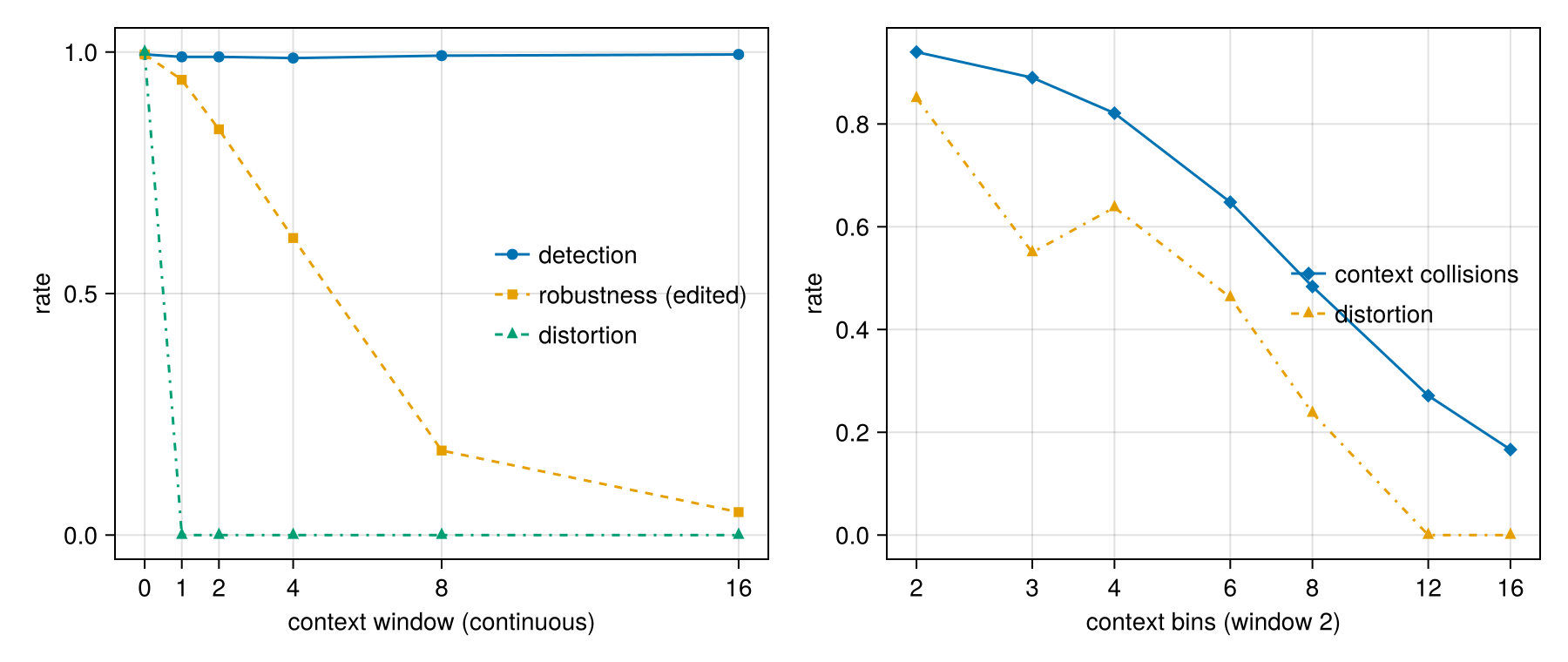
Now using the exact context suffers from adversarial edits: it affects not only that particular element but also the subsequent elements as it changes the context seeding. Thus the size of the context is important for the robustness to editing; the smaller the window the more robust we are to edits (since we get more unbroken sequences) but of course that also leads to more distortion. We can also try to fix the exactness problem by bucketing: if we use coarse buckets we have some hope of small edits not changing the bucket and thus not affecting our context.
Of course combining the two leads to more context collisions: the very problem we had with the fixed key! A production-level detector will need to tune these parameters to achieve good performance for its particular domain.
Power
Pulling it all together we can summarize our findings with a nice figure showing power as function of the sequence length:
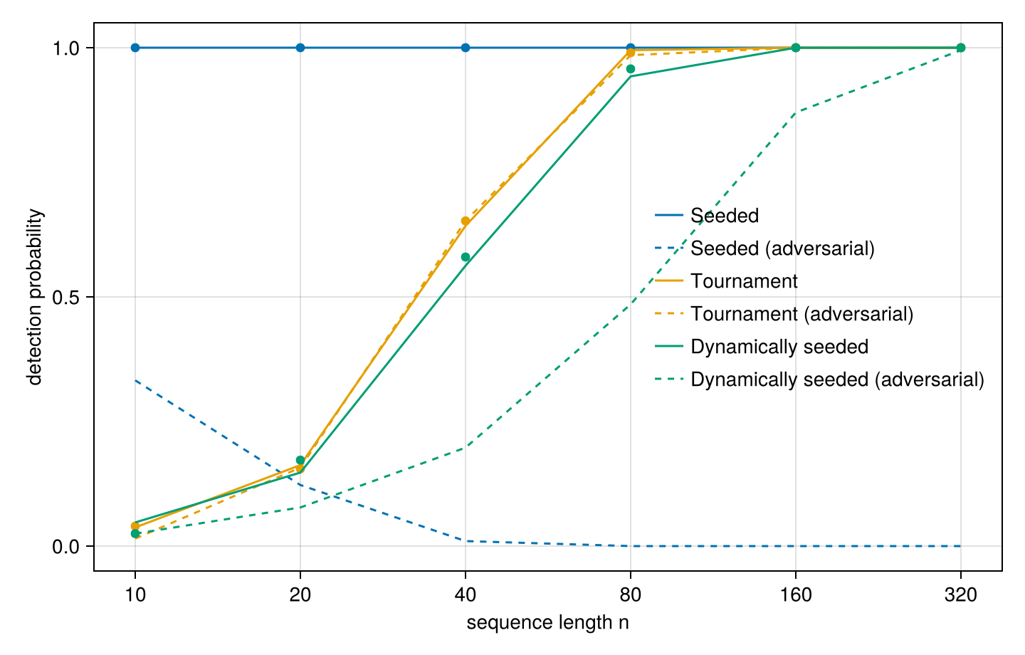
As expected every method asymptotes to one with more data. However we see differential impacts to editing: tournament is barely affected while we see stronger effects on the dynamically seeded; we do pay something for the multi-shot robustness.
We should note something interesting: the uniform distribution is literally the maximum-entropy distribution. Thus we have a ton of ability to introduce our watermark. What about something with far less entropy: say a Beta(200, 100)?
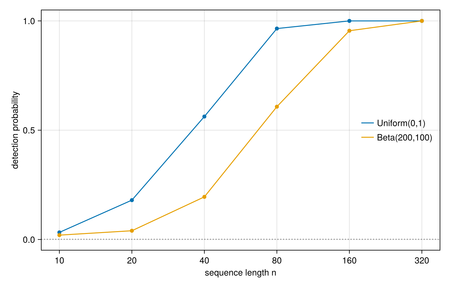
With this lower entropy distribution we have a way harder time: we need about twice as much data to detect our watermark without introducing a ton of distortion. Unfortunately this is the case for real LLM watermarking: it’s very hard to watermark low-entropy sequences like presumably code: often there is just the one right token otherwise the code wouldn’t run.
Conclusion
Thus it’s quite a hard problem. It seems better than classifier based approaches or adhoc witchhunts based on typography and vibes6. But of course there’s removal services7. Ultimately we might end up having to accept that there is no perfect way to detect LLM outputs and live with the consequences. That’s a much harder social problem than even the already hard technical problem.
-
Gotta love that em-dash troll ↩︎
-
Note that this lets you tell whether a particular model/generator created the output: it doesn’t solve the “was this output generated by any AI” unless everyone is using watermarks. Hence the EU’s regulation. ↩︎
-
Recommended reading list:
- Aaronson 2022
- Kirchenbauer et al. 2023
- Kuditipudi et al. 2023
- Christ, Gunn, Zamir 2023
- Dathathri et al. 2024
-
You should really set this based on the relative costs of type I (falsely accusing real text) vs type II (missing AI): depends on the context ↩︎
-
This obviously has to be the case otherwise what would the point be of more samples! ↩︎
-
Not that I can stop myself from speculating whenever I see an em-dash or other LLM-isms ↩︎
-
which seem to clearly be in violation of the EU’s regulation: they say any generator and the approach for removal is just paraphrasing with an unwatermarked LLM ↩︎