Asterisk has a fascinating article asking “Are Prediction Markets Good For Anything?” (spoiler: not much). This got me curious about the related question “Are Prediction Markets Good For Anyone?”. This naturally leads to a figure like this which plots the relative ROI (money won over money wagered) for a subsample of Polymarket accounts:
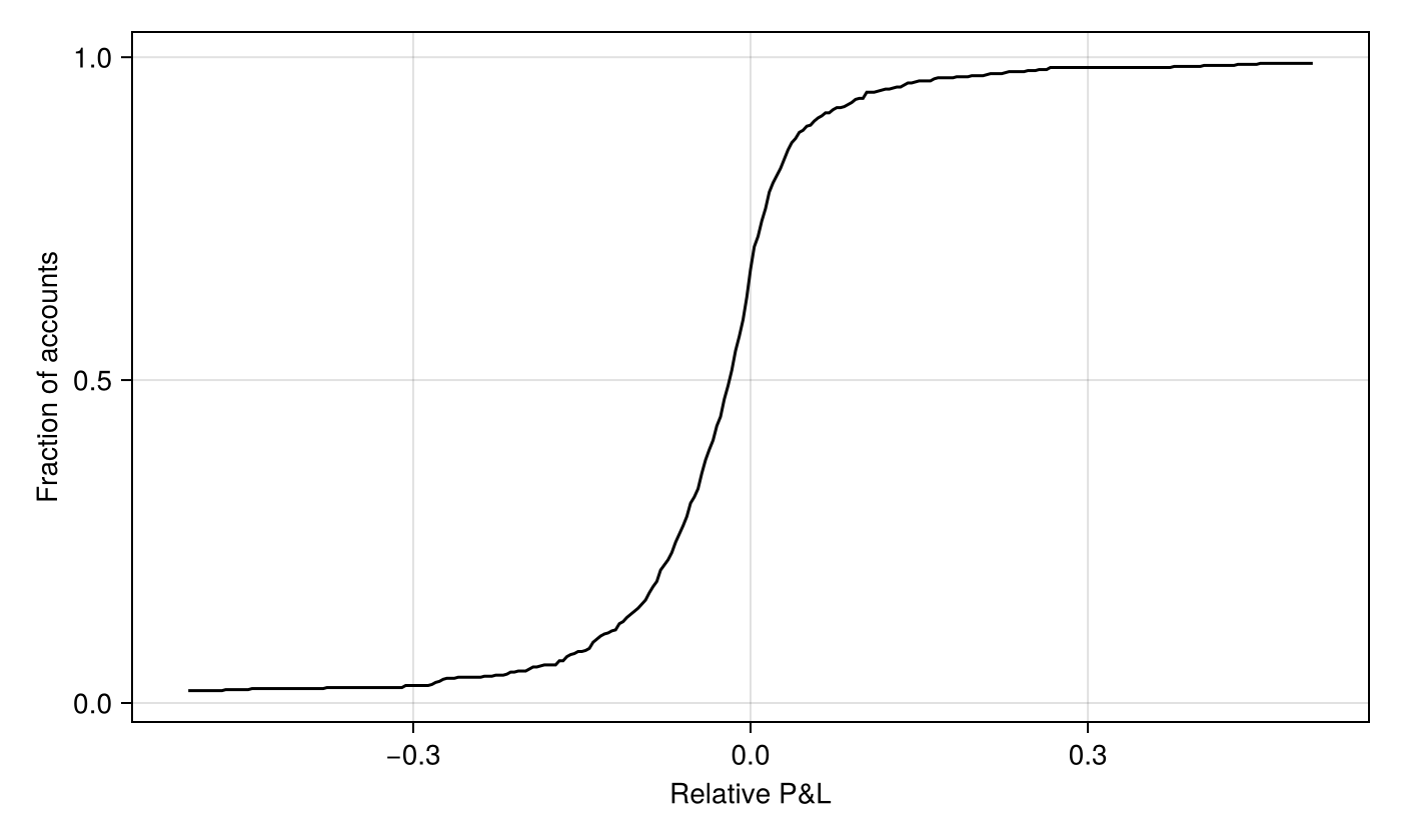
Figure 1: Cumulative distribution function for Polymarket returns by account
This figure shows that 14.7% of accounts have lost >= 10% of the money they’ve wagered. It’s quite tempting to conclude that these accounts are losers who would continue to lose >= 10% of their money going forward. Similarly we see that 6.4% of accounts have made >= 10% returns on their money: we might be tempted to see these accounts as having some inherent skill which will enable them to keep raking in >=10% on an ongoing basis.
Tempering the urge for this hasty conclusion is a four word explanation: “regression to the mean.” However on deeper look it gets even more interesting. After all we have lots of accounts: some exhibited outsized results due to noise but also some saw smaller results: surely an average over all accounts would cancel this out? And indeed an average would cancel; distributional quantities are different however and we need to make some careful adjustments.
Toy Example
Let’s start with a toy example: suppose the distribution of true effects is normally distributed \(\theta \sim N(0, 1)\). Our observations are noisy realizations: \(X_i = \theta_i + \epsilon_i\) where \(\epsilon_i \sim N(0, \sigma^2)\) independently of \(\theta_i\).
Let’s plot the observed distribution’s CDF for a couple different values of \(\sigma\) (dashed) on top of the true CDF (solid black).
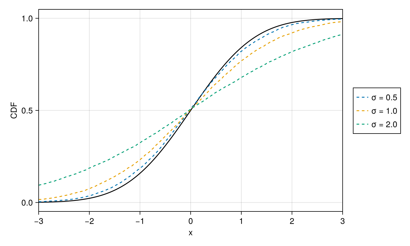
Figure 2: True (solid black) and observed (dashed) CDFs; noise causes systematic bias in the tails
You can clearly see the problem! Even though the noise is symmetric for every observation the tails are not! Indeed the outliers grow as σ increases: with no noise 15.9% of values exceed 1, at σ = 0.5 we observe 17.9% but by σ = 2.0 we observe 32.1%. In the limit as \(\sigma \rightarrow \infty\) this value would approach 50%.
To see why let’s consider a single point and how it contributes in expectation to the CDF evaluated at a point \(t\). In the noiseless case the observation contributes a step function \(\mathbf{1}\{\theta_i \le t\}\): nothing for \(t < \theta_{i}\) and its full weight of 1 for \(t \ge \theta_{i}\). In the noisy case however it contributes probabilistically: in expectation it contributes
\[P(X_i \le t) = \Phi\left(\frac{t - \theta_{i}}{\sigma}\right)\]
where \(\Phi\) is the standard normal distribution’s CDF. We can visualize the noiseless contribution (solid black) against the noisy contribution (dashed):
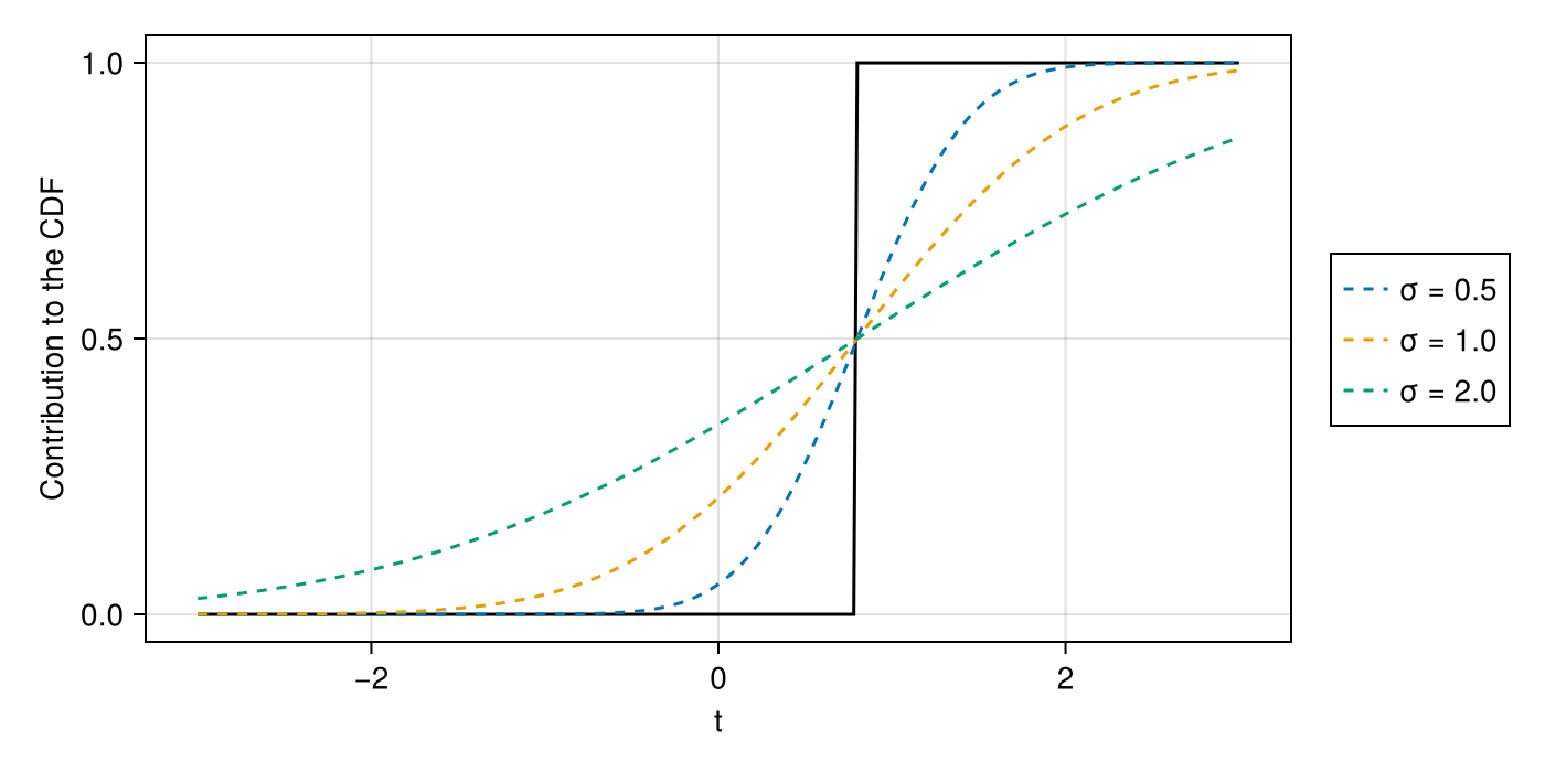
Figure 3: A single observation’s contribution to the CDF: the noiseless step (solid black) versus the smeared noisy contributions (dashed), which push mass into the tails.
Thus we see how the tails continue to grow. Averaging these contributions over the population shows the observed CDF is a convolution of the true CDF with the noise density:
\[F_X(t) = \int \Phi\left(\frac{t - u}{\sigma}\right) dF_\theta(u) = (F_\theta * \varphi_\sigma)(t)\]
Deconvolutions
But if we can convolve the distribution perhaps we can also deconvolve the distribution. Convolution is the easiest to understand in the frequency domain using the Fourier transform 1. In that domain convolution is then just a multiplication:
\[\psi_X(\omega) = \psi_\theta(\omega)\, \psi_\epsilon(\omega)\]
where \(\psi_\epsilon\) is the characteristic function of the noise. For our toy \(N(0, \sigma^2)\) noise this is \(\psi_\epsilon(\omega) = e^{-\sigma^2 \omega^2 / 2}\), which essentially acts as a low-pass filter: at low frequencies (\(\omega\)) it is close to 1 and as frequency increases it goes rapidly to zero.
With a known noise distribution we can undo the multiplication with a division: we estimate \(\psi_X\) by the empirical characteristic function, divide by \(\psi_\epsilon\), and invert back to a CDF.
But this causes some practical problems. Namely dividing by things that go rapidly to zero means that things now go rapidly to infinity. This is bad because our estimate of the empirical characteristic function has a sampling error of about \(O(1/\sqrt{n})\) at every frequency. And most smooth distributions decay as you go to higher frequencies which means at some point you’re multiplying mostly noise by huge numbers.
To avoid this we can do some truncation and zero out values where we’re mostly adding noise. Of course this now causes its own problems: removing all of the higher frequencies causes oscillations around sharp jumps. To avoid this we can do a soft taper instead (with a cosine but there’s plenty of alternatives).
Our final code looks like this
function deconvolve_cdf(x, σ, ts; T = sqrt(log(length(x))) / σ, m = 400)
    grid = range(T / m, T; length = m)
    ecf = [mean(cis.(t .* x)) for t in grid]
    amp = @. exp(σ^2 * grid^2 / 2)
    taper = @. (1 + cos(pi * grid / T)) / 2
    map(ts) do t₀
        gp = @. imag(cis(-grid * t₀) * ecf * amp) * taper / grid
        clamp(0.5 - sum(gp) * step(grid) / pi, 0, 1)
    end
end
Taking the \(\sigma = 0.5\) sample from above as our running example, we can deconvolve it with its known noise level. We plot each estimate’s error against the true CDF:
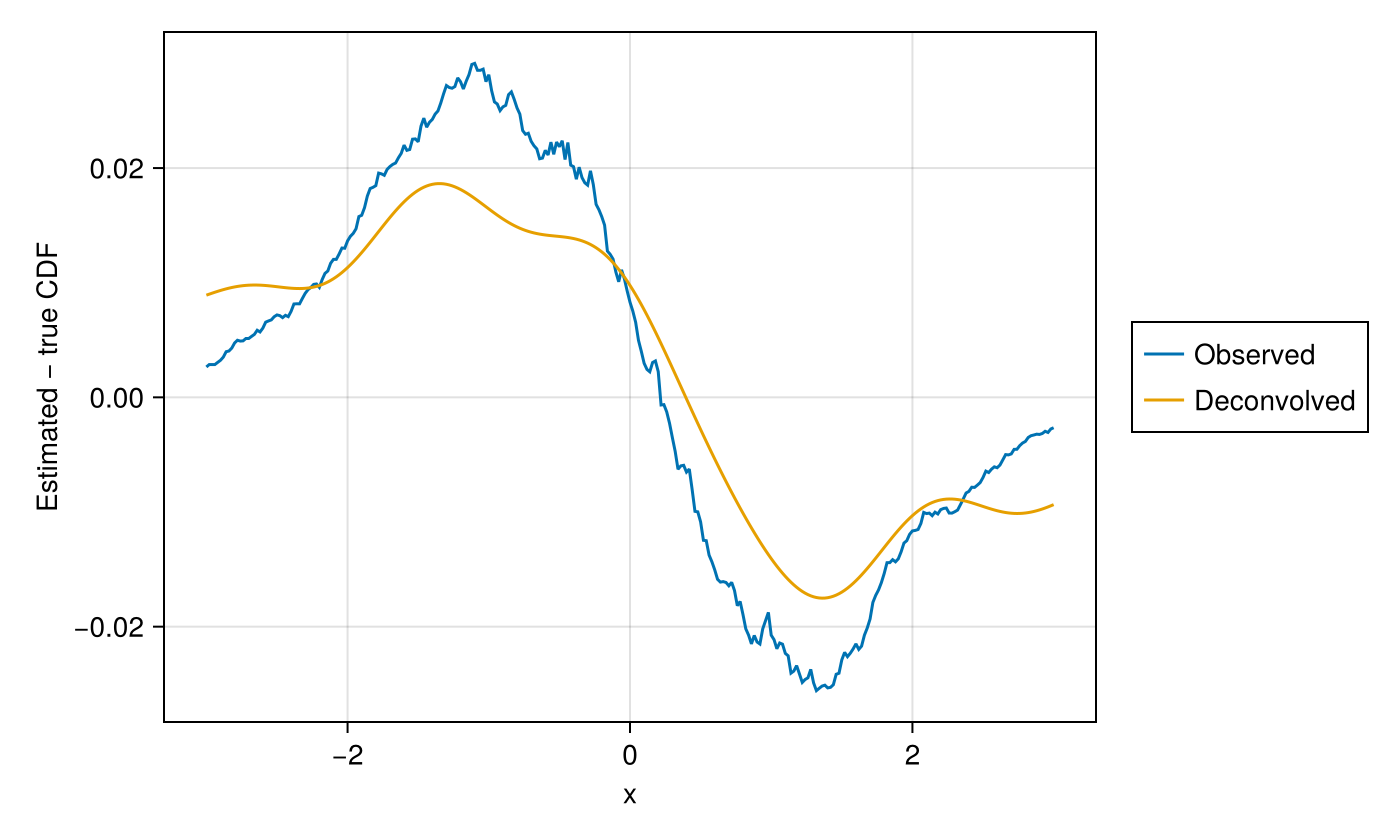
Figure 4: Error against the true CDF for the observed and deconvolved estimates ((sigma = 0.5)); deconvolution closes only part of the gap.
It helps, but less than you might hope: the deconvolution closes only part of the gap to the truth.
We can do the same thing with a different case: all true effects are 0
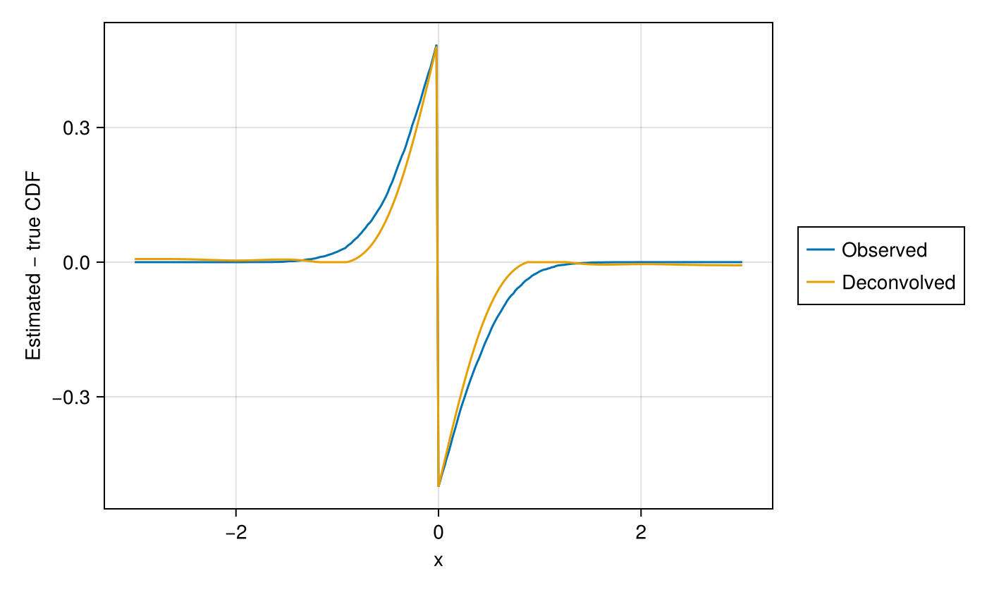
Figure 5: Same error view when every true effect is zero; deconvolution barely helps at the discontinuity.
Here we see even less of a benefit. This is a much harder distribution: the discontinuity requires arbitrarily high frequencies. Indeed its characteristic function has magnitude 1 at every frequency. Thus truncation is terrible; but, due to the noise and exponentially growing weights problem, not truncating is also terrible. In effect the convolution has destroyed some information here: the high frequencies are lost to the noise and we can’t reconstruct this distribution.
We can clearly see this in the frequency domain. We plot the magnitude of the recovered characteristic function against the true \(|\psi_\theta|\), together with the amplified sampling floor \(e^{\sigma^2\omega^2/2}/\sqrt{n}\) (note the log scale):
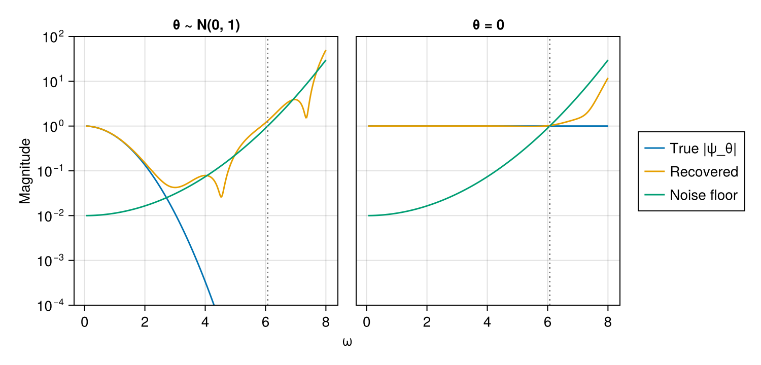
Figure 6: Recovered vs. true characteristic-function magnitude with the amplified sampling floor (log scale); the dotted vertical line marks the truncation frequency. The Gaussian’s coefficients vanish before the floor bites; the point mass’s do not.
In both panels the recovered coefficients track the truth until the noise overwhelms the true function. For the Gaussian on the left this costs little: by the time the floor takes over, the true coefficients are already negligibly small thus we can truncate (the vertical line) with no ill-effects (indeed we probably truncate too late). For the point mass on the right the true magnitude is 1 at every frequency so while we still match well the missing bits are missed.
The SIMEX algorithm
This is great but it relies on knowing the noise distribution exactly which we probably won’t know. Even worse each observation might have a different standard error, so it’s not even like we have a fixed noise distribution to deconvolve. Can we still do this?
SIMEX (SIMulation EXtrapolation), introduced by Cook and Stefanski 1994, approaches this in a fascinating manner. It takes the counterintuitive approach of adding even more noise to the data! The noise is carefully controlled and we measure the change in our estimates of interest relative to the magnitude of the noise. This is the simulation phase. We follow by an extrapolation phase which then extrapolates back to a noiseless state.
Let’s go through steps one by one. The key is to scale the added noise to each observation’s own measurement error: for a grid of values λ > 0 we generate pseudo-data
\[X_i(\lambda) = X_i + \sqrt{\lambda}\, \sigma_i\, \eta_{i}, \qquad \eta_{i} \sim N(0, 1)\]
so that \(X_i(\lambda)\) has total variance \((1 + \lambda)\sigma_i^2\). At \(\lambda = 0\) we recover the observed data, and larger \(\lambda\) inflates every observation’s noise by the same factor. We then estimate our parameter of interest using our new noisy distributions.
In the general algorithm we’d average over \(B\) independent draws of the \(\eta_{i}\) to wash out simulation noise, but for the CDF we can skip simulating entirely since the average over draws has a closed form:
\[E\left[\mathbf{1}\{X_i(\lambda) \le t\} \mid X_i\right] = \Phi\left(\frac{t - X_i}{\sqrt{\lambda}\, \sigma_i}\right)\]
which is the route Stefanski and Bay 1996 take for exactly this problem of debiasing the CDF.
We then plot the tail probability \(P(X > 1)\) as a function of \(\lambda\).
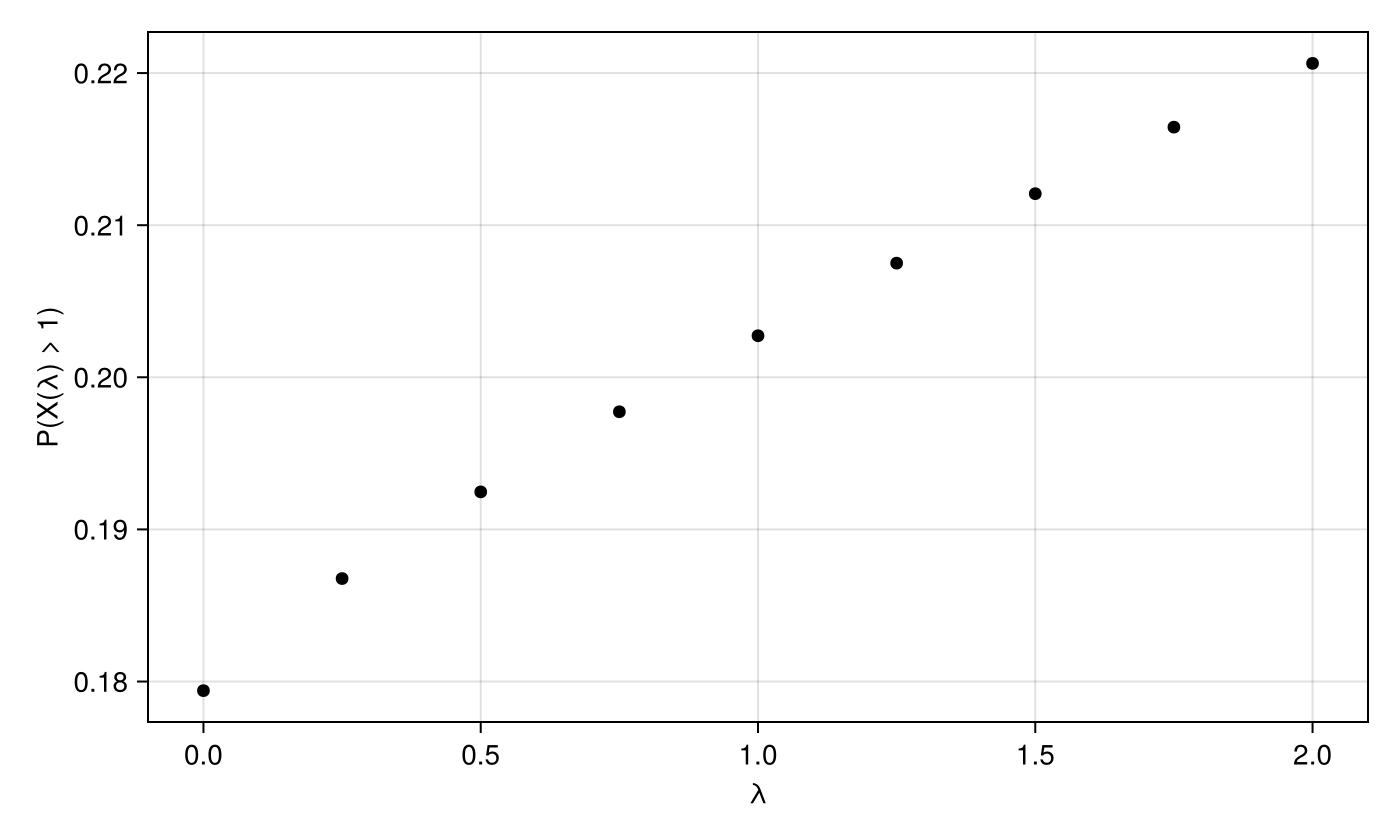
Figure 7: Observed tail probability (P(X(lambda) > 1)) as a function of the added-noise level (lambda).
This is remarkably smooth: we’ll model this as a quadratic (though to be fair it’s looking pretty linear here). We then extrapolate back to \(\lambda=-1\) which “zeros” out the noise.
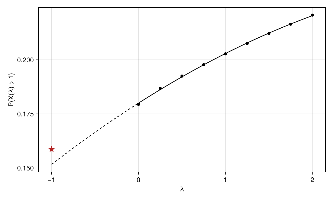
Figure 8: Quadratic fit to the simulated tail probabilities (solid), extrapolated to (lambda = -1) (dashed); the star marks the true value.
For this case it works well: the extrapolation lands at 15.2%, closing essentially all of the gap between the observed 17.9% and the true 15.9%. It even slightly overshoots the truth, but that is sampling error rather than a property of the method: this particular sample sits a little low overall (the exact noised tail at \(\lambda = 0\) is 18.6%), and the fitted curve inherits that shift. As we’ll see below, with no sampling error at all the truncated quadratic always lands short of the truth, somewhere between the observed value and the target.
Why does this work
The above was hopelessly handwavy so let’s start justifying this admittedly bizarre approach.
Denote \(\tau^2 = (1 + \lambda)\sigma^2\) as the total noise variance. Since \(X(\lambda) \le t\) exactly when \(\theta \le t - \tau Z\) for a standard normal \(Z\) independent of θ, the noised CDF is
\[G(t, \lambda) = E\left[F_\theta(t - \tau Z)\right]\]
We can Taylor-expand \(F_\theta\) around \(t\): the odd terms vanish with the odd moments of \(Z\), the even moments \(E[Z^{2k}] = (2k)! / (2^k k!)\) tidy up the factorials, and we are left with
\[G(t, \lambda) = E\ \sum_{k \ge 0} \frac{1}{k!} \left(\frac{(1+\lambda)\sigma^2}{2}\right)^k F_\theta^{(2k)}(t)\]
Evaluated at \(\lambda = -1\) every \(k \ge 1\) term is zero’d out, leaving exactly \(F_\theta(t)\): extrapolating to \(\lambda = -1\) is extrapolating to where the noise variance hits zero. The math for non-Gaussian noise is a little trickier but symmetric distributions also cancel out the odd terms.
We then truncate to the quadratic! Why quadratic rather than linear or some higher order? The exact function is an infinite-order Taylor expansion in \(\lambda\), so any truncated fit is biased. But adding additional terms adds variance and particularly quickly as sampling error in \(\hat{G}\) grows rapidly with the degree. Thus quadratic is the standard bias–variance compromise, and it is what Cook and Stefanski recommended.
This is actually a deconvolution
At first glance it’s not clear why I started this post talking about deconvolutions and Fourier space. And then we move to SIMEX which seems like it’s doing something completely different with sampling noise. But there is a payoff: for constant measurement error they’re basically doing the same thing!
Let’s examine what SIMEX does when estimating a single Fourier coefficient in the Gaussian case. SIMEX adds additional Gaussian noise so we now have a noise characteristic function \(e^{-(1+\lambda)\sigma^2\omega^2/2}\). Notice that this is just an exponential curve as a function of \(\lambda\).
So while in the deconvolution we somehow knew the characteristic function here we’re approximating the true exponential function with a lower order polynomial. And instead of dividing we just extrapolate to λ=-1 where this whole term becomes \(1\). A quadratic tracks \(e^{-(1+\lambda)\sigma^2\omega^2/2}\) well where \(\sigma^2\omega^2\) is small and poorly where it is large so as long as the approximation holds we’ve recovered the original characteristic function!
This also helps us understand the heteroskedastic case which was our original motivation. With observation-specific \(\sigma_i\) the observed distribution is no longer a clean convolution, so there is no single noise characteristic function by which to divide. But SIMEX doesn’t need the factorization: the exponential-in-λ identity holds for each observation simultaneously because we scaled each observation’s added noise to its own \(\sigma_i\).
Now of course we’re not actually fitting a Fourier component but some other functional.
But note that this must be a function of all of the Fourier coefficients simultaneously.
In our case the noised CDF at a single point can be written out with the Gil–Pelaez inversion formula (the same identity deconvolve_cdf implemented above):
\[G(t, \lambda) = \frac{1}{2} - \frac{1}{\pi} \int_0^\infty \mathrm{Im}\left[e^{-i\omega t}\, \psi_\theta(\omega)\right]\, e^{-(1+\lambda)\sigma^2\omega^2/2}\, \frac{d\omega}{\omega}\]
Thus the dependence on \(\lambda\) is not exactly an exponential but rather an integral of a bunch of exponentials, one per frequency, each weighted by the true Fourier coefficients. But this is helpful as the high frequency terms decay rapidly and thus our curve is dominated by the low frequencies which should be relatively well-behaved over the range of λ that SIMEX uses as we’ll see now.
How Much Can We Recover?
This decomposition helps us understand when and where SIMEX will work. The heart of SIMEX is an extrapolation, and extrapolations are always sketchy and usually fail quietly. To illustrate we can examine our normal example further. Take \(\theta \sim N(0, \tau^2)\), add noise \(\sigma\), compute the exact noised tail probability at every λ (no sampling error at all), fit the quadratic, and calculate the fraction of the observed-vs-true gap that the extrapolation recovers.
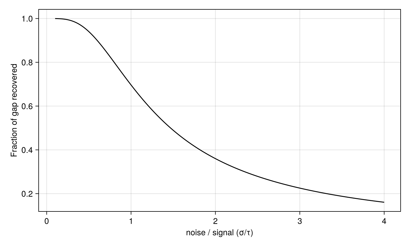
Figure 9: Fraction of the observed-vs-true gap recovered by the quadratic extrapolation as the noise-to-signal ratio grows (no sampling error anywhere).
There is no sampling error anywhere in this figure, so we’re just calculating the truncation bias. The quadratic cannot keep up with the exponential at \(\lambda = -1\), so the extrapolation always lands above the truth, between the observed value and the target.
Below \(\sigma \approx \tau\) the quadratic recovers essentially everything (at \(\sigma = \tau/2\) it closes 94.0% of the gap). By \(\sigma = 2\tau\) it closes only 36.0%, and at σ = 4τ just 16.1%. Once you get that far out you’ve recovered nothing, and the failure is silent: the extrapolated CDF looks exactly as smooth and plausible when it has recovered a sixth of the truth as when it has recovered all of it.
When we look at it through the lens of the Fourier approach we remember from the Gil-Pelaez formula that the CDF is an integral of the exponentials \(e^{-(1+\lambda)\sigma^2\omega^2/2}\) weighted by the true Fourier coefficients. When \(\sigma \ll \tau\) the true coefficients cut off the high frequencies and the exponentials that survive are relatively flat and easy to approximate and extrapolate. As \(\sigma\) grows relative to \(\tau\) the high frequencies still get cut off, but the surviving low-frequency components are now much sharper exponentials which are no longer well tracked by our quadratic. Thus SIMEX fails.
This framing also says the failure isn’t really about the signal to noise ratio per se. Rather it’s about the curvature of what we’re extrapolating: a quadratic tracks a gently bending \(G(t, \lambda)\) well but cannot follow the sharp exponentials that dominate once \(\sigma\) grows. And no better-chosen functional family fully saves it either, because \(G(t, \lambda)\) is not a single exponential but a mixture of them across frequencies.
Thus we can also break this by picking a different functional: say the density for instance! The CDF’s inversion integral damps frequency ω by \(1/\omega\), while the density’s does not; relative to the CDF it upweights exactly the high frequencies that the noise destroyed. Thus we start having noise problems again! The approaches are remarkably similar: a kernel density estimate with bandwidth \(h\) still has a closed form under added noise, since the extra noise just widens each kernel to \(\sqrt{h^2 + \lambda\sigma^2}\). Extrapolating it pointwise on our running example:
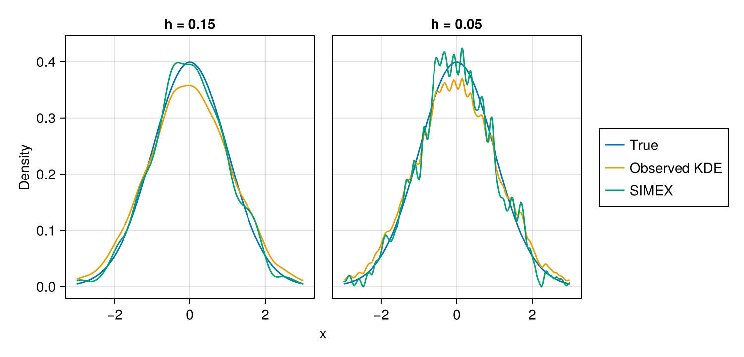
Figure 10: SIMEX applied to a kernel density estimate at two bandwidths: it corrects the bias but gets squiggly as the bandwidth shrinks and high frequencies are required.
SIMEX still fixes the bias as the extrapolated curve sits on the true density where the observed KDE is visibly too flat. But it comes back ragged, and the raggedness is not a sampling problem: it grows as the bandwidth shrinks. A smaller bandwidth emphasizes higher frequencies, and those are exactly the ones where the extrapolation is multiplying noise.
Calculating the whole CDF
All this was for calculating a single functional: what about evaluating the CDF on a grid of points? You might worry that as each point \(t\) gets its own quadratic there’s nothing tying neighboring extrapolations together. The extrapolated \(\hat{F}(t)\) can then dip below 0, exceed 1, or decrease in \(t\). And this totally happens, so we need a slight adjustment:
Instead of individual regressions we fit all of them together as one constrained least-squares problem. Stack the λ grid into the design matrix \(A\) with rows \((1, \lambda, \lambda^2)\), write \(\beta_j\) for the quadratic’s coefficients at grid point \(t_j\), and let \(e = (1, -1, 1)^\top\) so that \(e^\top \beta_j\) evaluates the quadratic at \(\lambda = -1\). For the grid \(t_1 < \dots < t_m\) we minimize the total error
\[\min_{\beta_1, \dots, \beta_m}\ \sum_{j} \left\| \hat{G}_j - A \beta_j \right\|^2 \quad \text{subject to } e^\top \beta_1 \le e^\top \beta_2 \le \dots \le e^\top \beta_m \text{ in } [0, 1]\]
where \(\hat{G}_j\) is the vector of noised CDF values at \(t_j\). The constraints are linear in the coefficients so this is a quadratic program.
We actually don’t need a QP solver though. Give the extrapolated value its own name, \(v_j = e^\top \beta_j\), and minimize in two stages: first over \(\beta_j\) with each \(v_j\) held fixed, then over the \(v_j\). The inner stage is least squares with a single linear constraint, and profiling it out has a nice closed form:
\[\min_{\beta_j:\ e^\top \beta_j = v_j} \left\| \hat{G}_j - A\beta_j \right\|^2 = \left\| \hat{G}_j - A\hat{\beta}_j \right\|^2 + w \left(v_j - \hat{v}_j\right)^2, \qquad w = \frac{1}{e^\top (A^\top A)^{-1} e}\]
where \(\hat{\beta}_j = (A^\top A)^{-1} A^\top \hat{G}_j\) is the unconstrained fit and \(\hat{v}_j = e^\top \hat{\beta}_j\) its extrapolation. Pinning the extrapolation incurs a quadratic penalty for moving away from the unconstrained answer, but it only depends on the \(\lambda\) grid and not on \(j\) or the data. Substituting into the joint objective, the residual terms are constants and the common \(w\) factors out, collapsing the outer stage to
\[\min_{v_1 \le \dots \le v_m}\ \sum_j \left(v_j - \hat{v}_j\right)^2\]
which is exactly an isotonic regression of the unconstrained extrapolations! Finally the \([0, 1]\) constraint comes for free: clamping a nondecreasing sequence keeps it nondecreasing, and clamping the isotonic fit is in fact the exact solution of the box-constrained problem.
Thus the final code is quite elegant:
using MultivariateStats: isotonic

function simex_cdf_unconstrained(x, σ, ts; λs = 0.0:0.25:2.0)
    G = [mean(cdf.(Normal.(x, sqrt(λ) .* σ), t)) for λ in λs, t in ts]
    coefs = [λ^p for λ in λs, p = 0:2] \ G
    return vec([1.0 -1.0 1.0] * coefs)
end

simex_cdf(x, σ, ts; λs = 0.0:0.25:2.0) =
    clamp.(isotonic(ts, simex_cdf_unconstrained(x, σ, ts; λs)), 0, 1)
where the isotonic regression is solved exactly. Note that \(\sigma\) can be a vector: each observation carries its own measurement error and the closed form broadcasts right through.
Toy Results
Let’s apply it to our two toy cases and plot the errors:
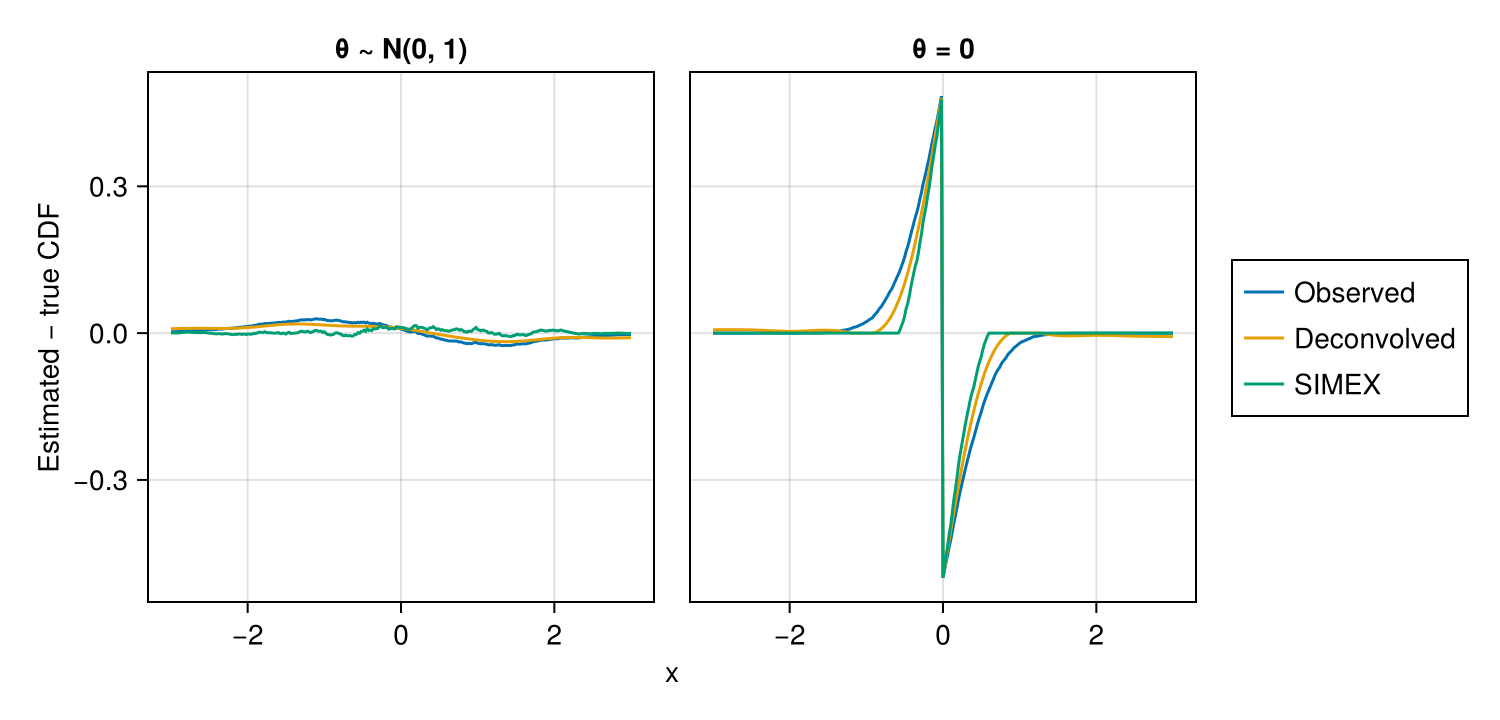
Figure 11: Error against the true CDF for the observed, deconvolved, and SIMEX estimates in the smooth and point-mass cases.
In the smooth case both SIMEX and the deconvolution shrink the error dramatically across the whole range, though SIMEX never needs the noise distribution that the deconvolution assumes. In the point-mass case they help less but SIMEX still performs slightly better.
So are Prediction Markets Good for Anyone
Coming back to the Polymarket example we see the following effect
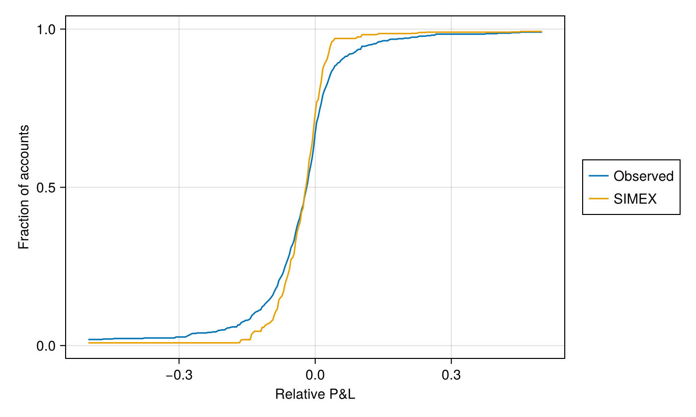
Figure 12: Observed versus SIMEX-corrected CDF of Polymarket account relative P&L; the corrected distribution is markedly narrower.
The corrected distribution is much tighter: the fraction of accounts down at least 10% falls from the observed 14.7% to 7.1%, and the fraction up at least 10% falls from 6.4% to 2.5%. Roughly half of each apparent tail is noise rather than persistent skill (or anti-skill).
We should be careful2 about what these estimates mean. Strictly speaking SIMEX doesn’t return us anything with strong statistical guarantees: we don’t achieve unbiasedness nor do we have consistency. With infinite data we’ll end up with a biased answer as sampling error will disappear but the truncation bias will remain.
Instead all we get is a slight narrowing of the bias in small samples for small noise levels. But this can still be useful and we can reason about the directionality of the errors which are conservative in this case.
For one we’ve got a reasonable signal-to-noise ratio: the typical account’s standard error is about 0.05, roughly 0.31 of the 0.17 spread across accounts. We’re around the part of the recovery curve where the quadratic closes almost the whole gap. By the same reasoning we know that the quadratic undershoots, so the SIMEX curve will still overstate the true spread: thus our number is more helpful interpreted as an upper bound.
Reassuringly, our estimates line up with some of the academic literature. Akey, Grégoire, Harvie and Martineau (2026) separate skill from luck, and reach a similar verdict from the opposite direction: rather than deconvolving a single cross-section, they split each trader’s bets and test out of sample, finding that roughly 60%3 of the apparent winners turn into losers on a fresh set of events.
Thus it seems reasonable to conclude that prediction markets (or perhaps more carefully just Polymarket) aren’t good for almost anyone except for a tiny fraction of users. And measuring those users is incredibly hard, and naive estimates will lead you astray.
-
which we statisticians call the characteristic function for some reason ↩︎
-
Cook and Stefanski write
When corrections for attenuation are made, they are often regarded by many with skepticism above and beyond the normal amount that should accompany any statistical modeling. The reason is that corrections for attenuation are often in the researcher’s best interest. For example, assuming that the presence of an effect has been convincingly demonstrated, the perceived importance of the effect is likely to depend on its magnitude. A correction for attenuation generally increases the magnitude of the effect; thus it is in the researcher’s interest to make such corrections.
…
In the situations just described, we believe that there is a need for corrections for attenuation that are both statistically and scientifically defensible while also being demonstratively conservative.
We’re in a slightly different position here as measurement error actually enhances the story: a shocking number of big winners and losers is far more exciting than mostly neutral. Which makes us have to argue even stronger for these corrections. ↩︎
-
this is the same ballpark as the fraction of the upper tail that SIMEX attributes to noise here, but don’t overindex on this: we have different populations and metrics. ↩︎