We’ve previously trained a neural network to predict which Pokemon will win a battle based on their stats. The motivation was tracking a Pokemon’s evolution: vanilla Bradley-Terry models would invalidate themselves but our model based on stats would still generalize well. Thus as a Pokemon levels up and evolves we can see how its probability of defeating an opponent rises.
This raises the natural question: what if we wanted to interfere with evolution and direct that development? In particular we might ask: which stats should we increase to have a reasonable chance of beating a particular boss?
For the normal leveling-up process we can just read the stats for each level and iterate until we achieve the requisite probability. In the directed case we need to be more clever as there’s many options we can choose. There is a topic from the ML fairness literature that is helpful here: individual recourse.
Individual Recourse
The original paper (as far as I can tell) to introduce the idea of recourse is Ustun 2019 (Actionable Recourse in Linear Classification). Their objective is:
\[ \min_{r} \; \mathrm{cost}( r) \quad \text{subject to} \quad \hat{f}(x + r) = t \]
That’s basically all you need to know. There’s a rather large literature1 but they all fundamentally are variations on this theme. This is somewhat obscured as many of the subsequent papers such as Wachter 2018 switch to a variant of the unconstrained/penalized version
\[ \min_{r} \; \mathrm{cost}( r) + \lambda \, (\hat{f}(x + r) - t)^{2} \]
This reformulation is a practical choice as it’s convenient to optimize. And of course it has a solution even when the original is infeasible. But ultimately it’s doing the same thing as \(\lambda \rightarrow \infty\) on satisfiable problems.
Thus we can summarize some of the literature as such:
| Paper | Objective | Optimizer |
|---|---|---|
| Ustun 2019 | cost | Integer programming |
| Wachter 2018 | cost | Gradient descent |
| REVISE (Joshi 2019) | Wachter in a latent space | Gradient descent |
| Dandl 2020 | + manifold / plausibility | Genetic search |
| DICE (Mothilal 2020) | + diversity across \(K\) solutions | Gradient / mixed |
We see that many of these papers simply modify the formula, adding some additional constraint targeting one of the -ities: sparsity2, plausibility, diversity, or causality.
This view helps make sense of the literature because the optimization algorithms are obscuring the nature of improvement. All of these choices between integer programming or gradient descent or spicier approaches like mixed optimization are more like implementation details. They fit the appropriate problem structure: like if you have neural networks gradients are cheap and easy while if everything is discrete then integer programming is the right way to go. We’ll indeed see this in our examples below.
Building out the data and model
Last time we used a Kaggle dataset of simulated battles. That’s enough for predicting, but here we want to act on the model’s advice and then check whether the advice was any good. So we need a battle engine we can query such as the open-source Pokemon Showdown engine.
For fights we’ll use the simulator’s built-in RandomPlayerAI.
This is noisy as expected and could be improved but that’s a whole other blog post.
We pit 730 pokemon against each other in 90000 battles creating a similar dataset as before.
On top of this data we retrain exactly the model from the previous post: a strength network plus an antisymmetric interaction term,
\[ P(a \text{ beats } b) = \sigma\!\big(\mathrm{strength}(x_a) - \mathrm{strength}(x_b) + \mathrm{SASNN}(x_a, x_b)\big), \]
where each \(x\) is the six stats and a one-hot encoding of the primary type.
Now that we have our data and our model let’s start investigating recourse!
Recourse for Pokemon
We’ll build up to four different versions of the cost:
| Version | What \(r\) may touch | \(\mathrm{cost}( r)\) | Optimizer |
|---|---|---|---|
| Unconstrained | any base stat, continuously | none (just need feasibility) | Gradient descent |
| Cost-aware | any base stat, continuously | \(\lVert r\rVert_2^2\) | Gradient descent |
| Diverse (DICE) | any base stat, continuously | + a diversity reward | Gradient descent |
| Realistic | the trainer’s levers (EV/IV/nat/L) | money | DFS branch-and-bound |
The unconstrained, cost-aware, and diverse versions share the same underlying optimization just with escalating costs. They work on the base statistics themselves which is a little unrealistic. To fix that we instead optimize on the set of levers actually available to a trainer and cost them according to the money required to buy the items causing those levers. Note that as we change the form of the problem we need to switch the optimization strategy: gradient descent works for the first two but the discrete nature of the realistic cost leads us to a depth-first search approach.
For our recourse target, let’s pick Magikarp, arguably the weakest Pokemon, and pit it against Mewtwo: one of the stronger pokemon. The model gives it essentially no chance in the baseline configuration; let’s figure out what we need to do to get Magikarp to a 50-50.
Unconstrained Recourse
We’ll treat the six stats as free continuous variables and fix the type (can’t change that). Let’s start by figuring out how we can get a single feasible point before starting to worry about the costs.
It’s actually rather easy: just projected gradient ascent on the predicted probability. The projection is there to keep us from going either negative or above a max value.
function unconstrained_recourse(
    attacker,
    defender;
    t = 0.5,
    lr = 0.05,
    n_steps = 6000,
    on_step = nothing,
)
    xa = feat(attacker)
    xd = feat(defender)
    Δ = zeros(Float32, N_FEATURES)
    fhat(d) = only(predict(full_model, xa .+ d, xd))

    p = fhat(Δ)
    on_step === nothing || on_step(0, Δ, p) # callback for tracing
    p >= t && return Δ

    for it = 1:n_steps # recourse may not be possible; hence finite steps
        prev = copy(Δ)
        g = Zygote.gradient(fhat, Δ)[1]
        Δ[1:N_STATS] .+= lr .* g[1:N_STATS] # only update the things that are not fixed
        Δ[1:N_STATS] .= clamp.(Δ[1:N_STATS], -xa[1:N_STATS], 1 .- xa[1:N_STATS])  # between 0 and 1 (normalized)
        p = fhat(Δ)
        on_step === nothing || on_step(it, Δ, p)
        if p >= t # crossed the line: bisect back to it
            lo = prev
            hi = Δ
            for _ = 1:40
                mid = (lo .+ hi) ./ 2
                fhat(mid) >= t ? (hi = mid) : (lo = mid)
            end
            return hi
        end
    end
    return Δ
end
We get the following recourse:
| Stat | Base | Change | Target |
|---|---|---|---|
| HP | 20 | +148 | 168 |
| ATK | 10 | +57 | 67 |
| DEF | 55 | +47 | 102 |
| SPA | 15 | +25 | 40 |
| SPD | 20 | +90 | 110 |
| SPE | 80 | +28 | 108 |
| P(win) | 0.001 | 0.5 |
Thus we find that we have to increase our statistics by a huge amount over 8x-ing HP and 5x-ing SPD to survive the fight. Attack is not that emphasized which is interesting: this is more of a turtle strategy.
It’s also informative to look at the path our optimization took:
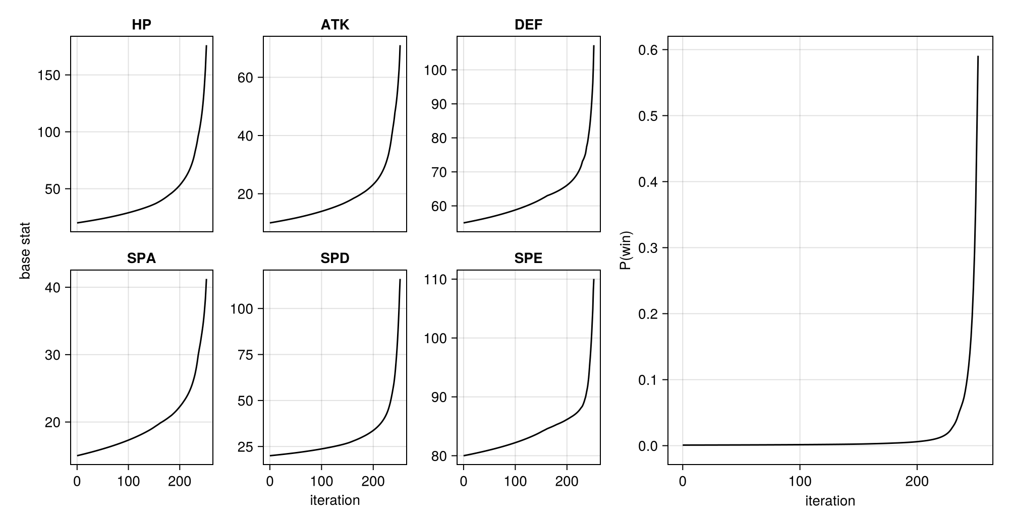
We started a long way away from the target and it was basically flat for almost all of the time until finally cresting at the finish. We needed the gradient information from the model to do this: if we had to increase the stats manually and actually compete to find out if progress had been made this would have taken forever.
Cost Aware Recourse
So we know there’s at least a feasible solution; let’s now consider cost. We’ll use the usual L2 norm penalty:
\[ \min_{r} \; \lVert r\rVert^2 + \lambda\,(\hat{f}(x+r) - t)^2 \]
when \(\lambda\) is large we pin the solution on the boundary and then the \(\lVert r\rVert^2\) component keeps the norm small. This preferentially chooses recourse which moves all of the stats a little rather than one stat a lot (assuming both hit feasibility).
function min_norm_recourse(
    attacker,
    defender;
    t = 0.5,
    λ = 1000,
    lr = 0.02,
    n_steps = 8000,
    clip = 0.02,
)
    xa = feat(attacker)
    xd = feat(defender)
    fhat(d) = only(predict(full_model, xa .+ d, xd))
    loss(d) = sum(abs2, d[1:N_STATS]) + λ * (fhat(d) - t)^2
    Δ = zeros(Float32, N_FEATURES)
    for _ = 1:n_steps
        g = lr .* Zygote.gradient(loss, Δ)[1][1:N_STATS]
        m = maximum(abs, g)
        m > clip && (g .*= clip / m)
        Δ[1:N_STATS] .-= g
        Δ[1:N_STATS] .= clamp.(Δ[1:N_STATS], -xa[1:N_STATS], 1 .- xa[1:N_STATS])
    end
    # project exactly onto f̂ = t to be comparable with unconstrained
    for _ = 1:50
        err = fhat(Δ) - t
        abs(err) < 1.0f-4 && break
        gg = Zygote.gradient(fhat, Δ)[1][1:N_STATS]
        Δ[1:N_STATS] .-= (err / (sum(abs2, gg) + 1.0f-8)) .* gg
        Δ[1:N_STATS] .= clamp.(Δ[1:N_STATS], -xa[1:N_STATS], 1 .- xa[1:N_STATS])
    end
    return Δ
end
| Stat | Base | Change | Target |
|---|---|---|---|
| HP | 20 | +134 | 154 |
| ATK | 10 | +52 | 62 |
| DEF | 55 | +58 | 113 |
| SPA | 15 | +20 | 35 |
| SPD | 20 | +98 | 118 |
| SPE | 80 | +36 | 116 |
| P(win) | 0.001 | 0.5 | |
| ‖r‖₂ (vs ascent) | 0.924 | 0.917 |
Interestingly there’s not a ton of difference from unconstrained and the cost is roughly the same (though a little smaller).
Diverse recourse
Of course if you don’t want to go that particular route you’re a bit at a loss. It would be nice if we instead gave you a couple options: you could then opt for the build that matches your own preferred play style.
Of course if we do this optimization a couple times we’ll get the same result. We could add a stochastic component but even then we’re likely to wind up in the same basin3. No, to get diverse solutions we’ll need to optimize for it directly.
We’ll start with k potential recourses and then maximize a pairwise distance
\[ \max_{r_1,\dots,r_K}\; \sum_{k<l}\lVert r_k - r_l\rVert_2^2 \quad\text{s.t.}\quad \hat{f}(x + r_k) = t,\ \; r_k \ge 0. \]
Instead of looking for a min-norm we’re now looking for K different recourses which all land on the boundary \(\hat{f}(x + r_{k}) = t\) but which are as spread out as far as possible. We need to add a new constraint \(r_{k} \ge 0\) as otherwise we’d start recommending decreasing stats to become even more diverse. Note we could have kept the min-norm penalty to get both diversity as well as avoiding huge changes but for didactic purposes we’ll drop it.
We solve this in two steps: the first with a diversity step which does gradient ascent on the pairwise distance penalizer. This knocks the solution off the boundary so we then project it back onto the boundary with a ray search. We seed our search at jittered copies of the unconstrained plan and iterate from there.
function dice_directions(
    attacker,
    defender;
    K = 3,
    t = 0.5,
    λd = 0.05,
    n_steps = 1200,
    seed = 1,
)
    Random.seed!(seed)
    xa = feat(attacker)
    xd = feat(defender)
    hi = 1 .- xa[1:N_STATS]
    padded(v) = vcat(v, zeros(Float32, n_types))

    function project(u)
        # we do a ray search since our model is approximately monotonic
        uc = max.(u, 0)
        sum(uc) <= 0 && return zeros(Float32, N_STATS)
        f(a) = only(predict(full_model, xa .+ padded(min.(a .* uc, hi)), xd))
        ahi = 1.0f0
        while f(ahi) < t && ahi < 1.0f7
            ahi *= 2
        end   # bracket the boundary
        f(ahi) < t && return min.(ahi .* uc, hi)                     # unreachable even maxed
        alo = 0.0f0
        for _ = 1:40
            am = (alo + ahi)/2
            f(am) >= t ? (ahi = am) : (alo = am)
        end
        min.(ahi .* uc, hi)
    end

    # start from K jittered copies of the unconstrained plan, each on the boundary
    Δu = max.(unconstrained_recourse(attacker, defender, t = t)[1:N_STATS], 0.0f0)
    cols = [project(Δu .+ 0.15 .* abs.(randn(Float32, N_STATS))) for _ = 1:K]
    spread(M) = sum(sum(abs2, M[:, k] .- M[:, l]) for k = 1:K for l = 1:K if k < l)
    for _ = 1:n_steps
        M = reduce(hcat, cols)
        g = Zygote.gradient(spread, M)[1]          # ascend the pairwise-distance reward
        for k = 1:K
            cols[k] = project(cols[k] .+ λd .* g[:, k])
        end  # push apart, re-project onto the boundary
    end
    return reduce(hcat, cols)
end
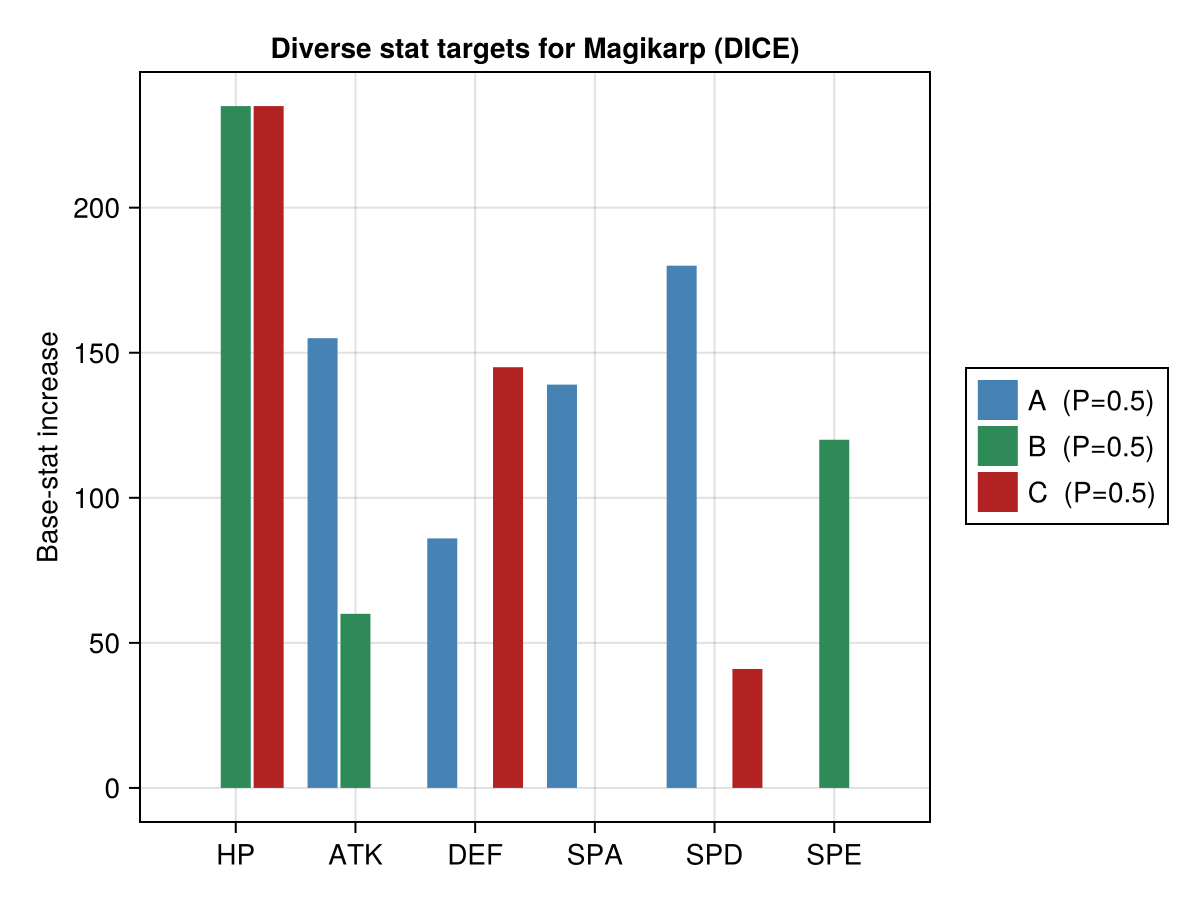
We find three options from this:
- A doesn’t touch HP at all and just invests heavily in ATK and SPA to get damage in while investing in SPD and to a lesser extent DEF for survivability.
- B on the other hand ignores DEF and SPD altogether and jacks up HP to survive and uses SPE and some ATK to get licks in.
- C joins B in beefing up HP but then turtles even harder investing in DEF and SPD.
You can obviously see the gameplay style implications: this is a nice touch to give a choose-your-own-adventure flavor to recourse.
Recourse with realistic costs
Of course, some of these are not actually achievable in-game. Aside from cheating, you only have basically four ways to increase stats: EVs (<=252/stat, 510 total), IVs (0-31), a nature (+/-10%), and level.
We can relate these to the base statistics (at level 50) with the following code:
# stat order: 1 hp, 2 atk, 3 def, 4 spa, 5 spd, 6 spe
is_hp(statidx) = (statidx == 1)
function actual_stat(base, iv, ev, level, nature, statidx)
    core = fld((2base + iv + fld(ev, 4)) * level, 100)
    return is_hp(statidx) ? core + level + 10 : floor(Int, (core + 5) * nature)
end

const NATURE_NAME = Dict(
    (0, 0)=>"Serious",
    (2, 3)=>"Lonely",
    (2, 4)=>"Adamant",
    (2, 5)=>"Naughty",
    (2, 6)=>"Brave",
    (3, 2)=>"Bold",
    (3, 4)=>"Impish",
    (3, 5)=>"Lax",
    (3, 6)=>"Relaxed",
    (4, 2)=>"Modest",
    (4, 3)=>"Mild",
    (4, 5)=>"Rash",
    (4, 6)=>"Quiet",
    (5, 2)=>"Calm",
    (5, 3)=>"Gentle",
    (5, 4)=>"Careful",
    (5, 6)=>"Sassy",
    (6, 2)=>"Timid",
    (6, 3)=>"Hasty",
    (6, 4)=>"Jolly",
    (6, 5)=>"Naive",
)
nature_choices() = collect(keys(NATURE_NAME))

function nature_vec(pj, mj)
    ν = ones(Float32, N_STATS)
    pj > 0 && (ν[pj] = 1.1; ν[mj] = 0.9)
    return ν
end

function levers_to_x(name, IVs, EVs, ν, L)
    a = [actual_stat(base_of(name)[j], IVs[j], EVs[j], L, ν[j], j) for j = 1:N_STATS]
    return to_input(a, type1_of(name))
end
The costs vary as well; interestingly, we can actually price them in terms of the in-game currency. In code we have
const EV_YEN = 1_000 # a Vitamin gives +10 EV
const MINT_YEN = 20_000 # one Mint buys any non-neutral nature
const CAP_YEN = 20_000 # a Bottle Cap Hyper-Trains one IV to 31
const CANDY_YEN = 3_000 # nominal ₽ per XL Exp. Candy (30k XP)

# Leveling isn't linear: total XP follows the Slow growth group for Magikarp
# xp(L) = 1.25·L³, so each successive level costs progressively more candies.
candies_to(L) = ceil(Int, max(0, 1.25 * L^3 - 1.25 * Lstar^3) / 30_000)
level_cost(L) = candies_to(L) * CANDY_YEN

function lever_cost(EVs, nature, IVs, L)
    ev = sum(EVs) * EV_YEN
    nat = nature == (0, 0) ? 0 : MINT_YEN
    iv = sum(IVs .== 31) * CAP_YEN
    lvl = level_cost(L)
    (ev = ev, nature = nat, iv = iv, level = lvl, total = ev + nat + iv + lvl)
end
To optimize this we need to consider discrete choices. Thus we need to change up our optimization from gradient descent.
We’ll use depth-first search but we’ll need to do a little pruning. Level is our biggest factor and for some levels it’s simply not possible to achieve our target win probability. We can check this by maxing out every stat as an optimistic upper bound: if that doesn’t achieve the target then we assume nothing can. Now that’s not exactly true since we can have non-monotonicity in our model but it’s a reasonable heuristic.
function stat_gains(attacker, defender, IVs, ν, L; ev_step = 10)
    xd = feat(defender)
    map(1:N_STATS) do j
        e = zeros(Int, N_STATS);
        e[j] = ev_step
        only(predict(full_model, levers_to_x(attacker, IVs, e, ν, L), xd))
    end
end

function greedy_cost(
    attacker,
    defender,
    IVs,
    ν,
    L;
    t = 0.5f0,
    ev_total = 510,
    ev_cap = 250,
    ev_step = 10,
)
    xd = feat(defender)
    EVs = zeros(Int, N_STATS)
    pcur = only(predict(full_model, levers_to_x(attacker, IVs, EVs, ν, L), xd))
    while sum(EVs) + ev_step <= ev_total && pcur < t
        bj = 0
        bp = pcur
        for j = 1:N_STATS
            EVs[j] + ev_step <= ev_cap || continue
            EVs[j] += ev_step
            p = only(predict(full_model, levers_to_x(attacker, IVs, EVs, ν, L), xd))
            EVs[j] -= ev_step
            p > bp && (bp, bj = p, j)
        end
        bj == 0 && break
        EVs[bj] += ev_step
        pcur = bp
    end
    pcur >= t ? EVs : nothing
end

function realistic_recourse(
    attacker,
    defender;
    t = 0.5f0,
    Lmax = 100,
    ev_cap = 250,
    ev_step = 10,
)
    IVs = fill(31, N_STATS)
    xd = feat(defender)
    ivcost = sum(IVs .== 31) * CAP_YEN
    best = Ref(Inf)
    bestsol = Ref{Any}(nothing)
    pwin(ν, L, EVs) = only(predict(full_model, levers_to_x(attacker, IVs, EVs, ν, L), xd))

    for L = Lmax:-5:Lstar, (pj, mj) in nature_choices()
        fixed = level_cost(L) + ivcost + (pj == 0 ? 0 : MINT_YEN)
        fixed >= best[] && continue                              # cheapest possible build too pricey
        ν = nature_vec(pj, mj)
        pwin(ν, L, fill(ev_cap, N_STATS)) >= t || continue       # optimistic ceiling: unreachable even maxed

        function record!(EVs)
            best[] = fixed + sum(EVs) * EV_YEN
            bestsol[] = (
                p = pwin(ν, L, EVs),
                EVs = copy(EVs),
                IVs = IVs,
                nature = (pj, mj),
                L = L,
                cost = sum(EVs),
                yen = best[],
            )
        end

        # greedy feasible build → tighten the ₽ incumbent cheaply before the exact search
        gEV = greedy_cost(
            attacker,
            defender,
            IVs,
            ν,
            L,
            t = t,
            ev_cap = ev_cap,
            ev_step = ev_step,
        )
        gEV !== nothing && fixed + sum(gEV) * EV_YEN < best[] && record!(gEV)

        # exact DFS: pile whole vitamins onto the highest-gain stats first, pruning any
        # partial build whose running ₽ already meets the incumbent
        cand = sortperm(
            stat_gains(attacker, defender, IVs, ν, L, ev_step = ev_step),
            rev = true,
        )
        EVs = zeros(Int, N_STATS)
        function dfs(ci)
            fixed + sum(EVs) * EV_YEN >= best[] && return
            pwin(ν, L, EVs) >= t && return record!(EVs)
            for i = ci:N_STATS
                j = cand[i]
                EVs[j] + ev_step <= ev_cap || continue
                EVs[j] += ev_step
                dfs(i)
                EVs[j] -= ev_step
            end
        end
        dfs(1)
    end
    bestsol[]   # nothing if unreachable
end
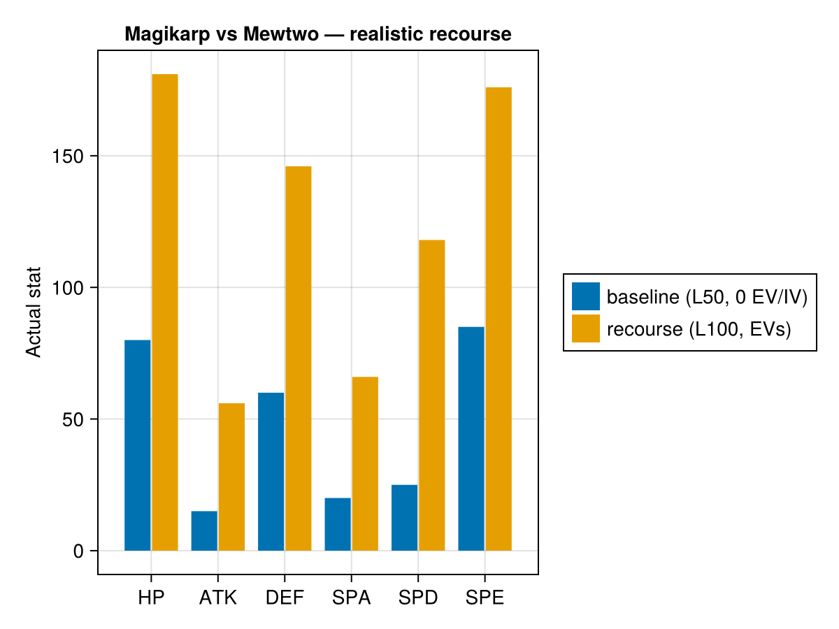
| Lever | Setting |
|---|---|
| Level | 100 |
| Nature | Sassy |
| IVs | all 31 |
| ATK EVs | 10 |
| SPD EVs | 120 |
| Total EVs | 130 |
| Cost (₽) | 381000 |
Does the advice actually work?
The whole point of this exercise was to get Magikarp to an even match with Mewtwo. We’ve got a bunch of different recommended builds which all achieve this in the model: let’s see if this holds true in the engine.
| Plan | Model P(win) | Real win rate |
|---|---|---|
| baseline | 0.001 | 0.0 |
| unconstrained | 0.5 | 0.04 |
| min-norm | 0.5 | 0.01 |
| dice 1 | 0.5 | 0.16 |
| dice 2 | 0.5 | 0.005 |
| dice 3 | 0.5 | 0.0 |
| realistic | 0.502 | 0.53 |
And they very much do not! Only the realistic succeeds; the others have pitiful chances.
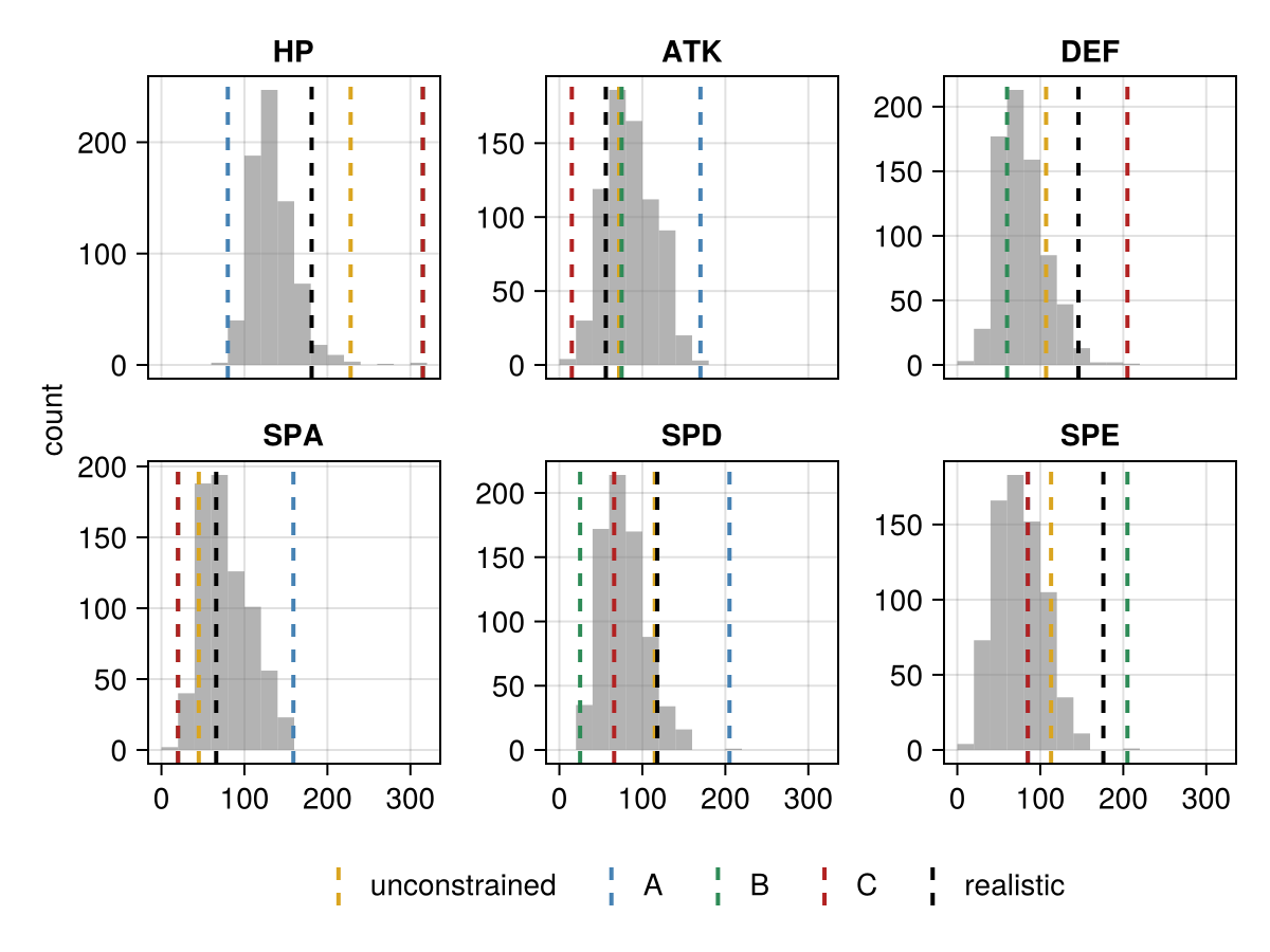
It’s informative to understand why: when you look at the distribution of observed stats you find that the other recourse options have stats which are well into the tail of the distributions. The model is extrapolating off its training distribution and thus is not going to perform well.
Of course there could be another reason why the plans fail. We’ve forgot about causality! Stats are not the whole story and the model can only see stats. Our boosted Magikarp still has very weak moves: Splash and Tackle. We have a clear unobserved confounder: it’s rather remarkable we achieved the 50-50 win rate! If we had removed Tackle it’d be even worse!
More generally all of this recourse speaks only to the model: we can deterministically flip the verdict not the underlying probability of the event.
You could see this clearly if we had some variable like battle_win_rate which obviously is correlated with winning more.
We can juice it by beating up on a weak Pokemon.
Doing so (and nothing else) would of course do nothing for our probability of winning.
This is exactly the causal recourse problem, and you see it in the wild all the time: Volkswagen realizing it only needed to reduce its testing emissions, or teachers realizing they just need to teach to the test.
This leads to an interesting conundrum: does providing recourse to individuals break the ability to use the model? Covariates which were merely correlational are still useful for prediction. But only if they’re not gamed (see König et al 2025). Recourse though basically tells us which variables to game thus we have to only use causal variables. But, of course, if we had a reliable causal model we’d already be using it. It kind of makes you want to adopt the Oracle of Delphi method and have your recourse be very cryptic: instead of telling folks “increase the average age of your credit cards” we should tell them “wisdom comes with experience beware the new”. Then maybe they’ll improve their credit without learning exactly what the model is looking for?
-
You’ll notice that this is exactly the same formulation as the original adversarial examples paper! They just use \(||r||_{2}\) as the cost. Only the intent is different: for adversarial examples instead of making recourse cheaper you’re actually trying to make recourse very costly! ↩︎
-
It’s not clear to me that you want sparsity. The Ustun paper makes the remark that if you have one unconstrained feature you always have recourse by just jacking that value to infinity. Which seems like you are going to overfit. ↩︎
-
This raises the natural question: is this a convex problem? If yes then you’d always end up in the same place. For certain models I think this could hold but in general no. The set of points which satisfy our target is not necessarily convex: you can have many different local optima around which disjoint neighborhoods all satisfy the constraint. Even if you have just a single global optimum your superlevel sets need not be convex either ↩︎