The challenge of detecting GenAI content via tools like Pangram gives rise to a fascinating statistical question: how can you tell if your detection is working, when you yourself can’t tell?
Like the typical way you would do this is to collect a bunch of examples, label them as real or GenAI, and then calculate your detector’s precision and recall. But, um, the whole point of needing a detector is that you don’t already have a reliable way of telling whether something is real or GenAI!
You’re in a bit of a pickle then: really the only way to verify that something is real or GenAI is to create it yourself. And it’s not like anyone wants to slave away making a bunch of real stuff every time they want to measure detector performance. You could try to scrape the internet but that’s probably mostly GenAI now. Really the only easy thing to do is collect a GenAI examples. So you’re stuck in an awkward position with a set of true positives and a whole lot of examples with uncertain provenance.
Surely you’re out of luck right?
It turns out: you can actually recover the whole classifier performance, as if you had the labels (under some assumptions). There’s even a whole literature about these problems: positive-unlabelled learning!
Positive Unlabelled Learning
The primary focus of the field1 is on fitting the classifier in the first place. The central insight is that it’s (often) perfectly fine to learn classifiers separating a pure positive distribution from a mixed positive and negative distribution. Your class prior probabilities get messed up but often your decision boundaries are equivalent.
You can see this in the following figure: we get a nice decision boundary with fully observed labels. But supposing we get to keep our positives but also get a mixture of positives and negatives in an unlabelled data set we learn basically the same shape of decision boundary just slightly shifted (depending on the relative size of the two sets).
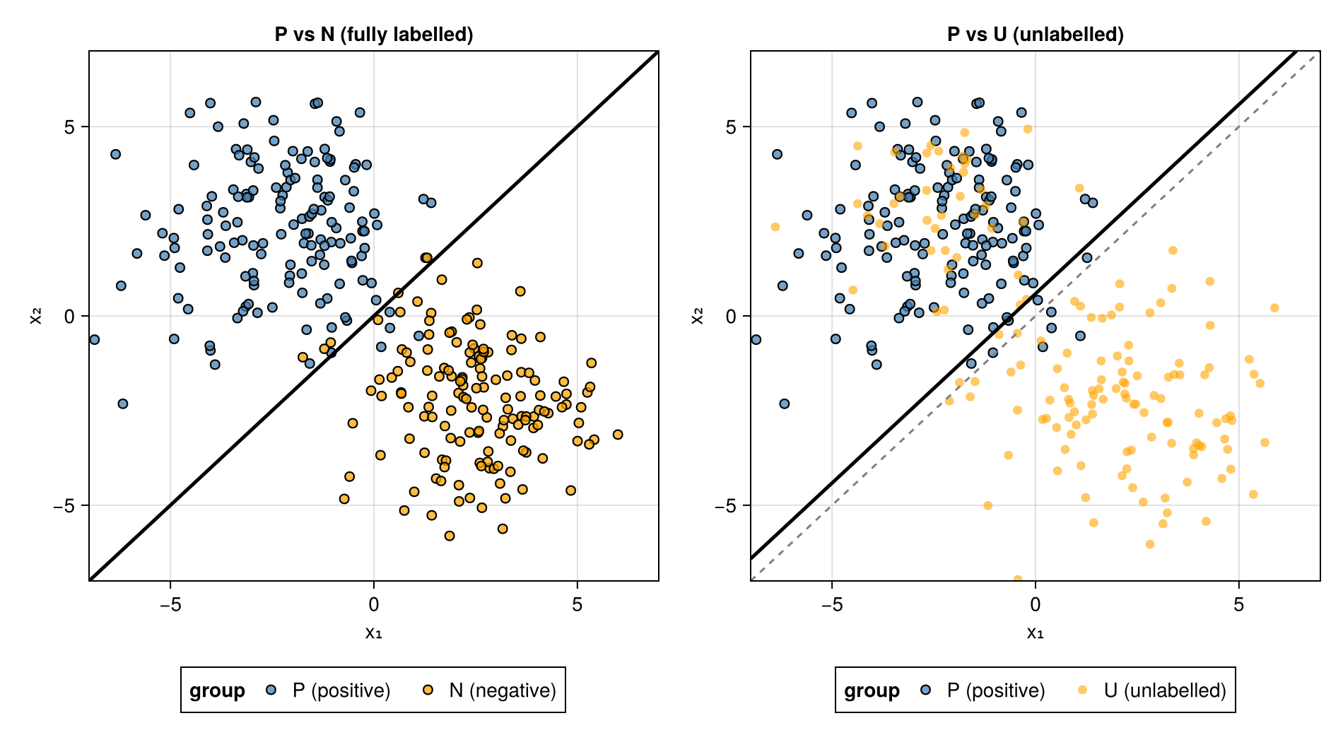
The most important assumption is that the positive distribution is the same between your labelled and unlabelled data. Which is certainly not trivial but remember we’re working in a fairly tight spot: we need to make (and check) these assumptions to get anywhere without access to negatives.
The rest of the field is mostly just finding ways to relax this in interesting ways: for instance Learning from Positive and Unlabeled Data with Arbitrary Positive Shift just requires you to have the negative class stay consistent:
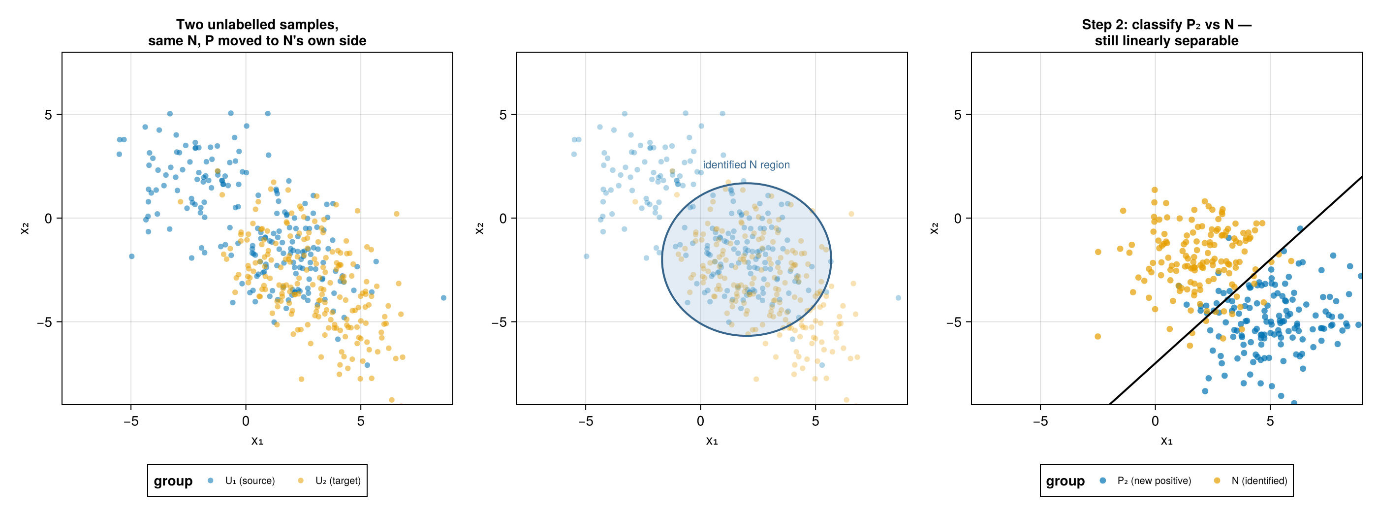
Very cool stuff but now let’s focus on our particular subproblem: no matter how you fit your classifier, now you need to estimate its performance!
Classifier Performance
\[ U = \alpha P + (1 - \alpha)N \]
where \(\alpha\) is the mixing proportion, \(P\) the positive distribution, and \(N\) the negative distribution.
Note that we have no idea about what \(N\) could be: we only have negatives in our unlabelled data and are unable to obtain labels for these points. All we have that’s observed is \(U\) and \(P\).
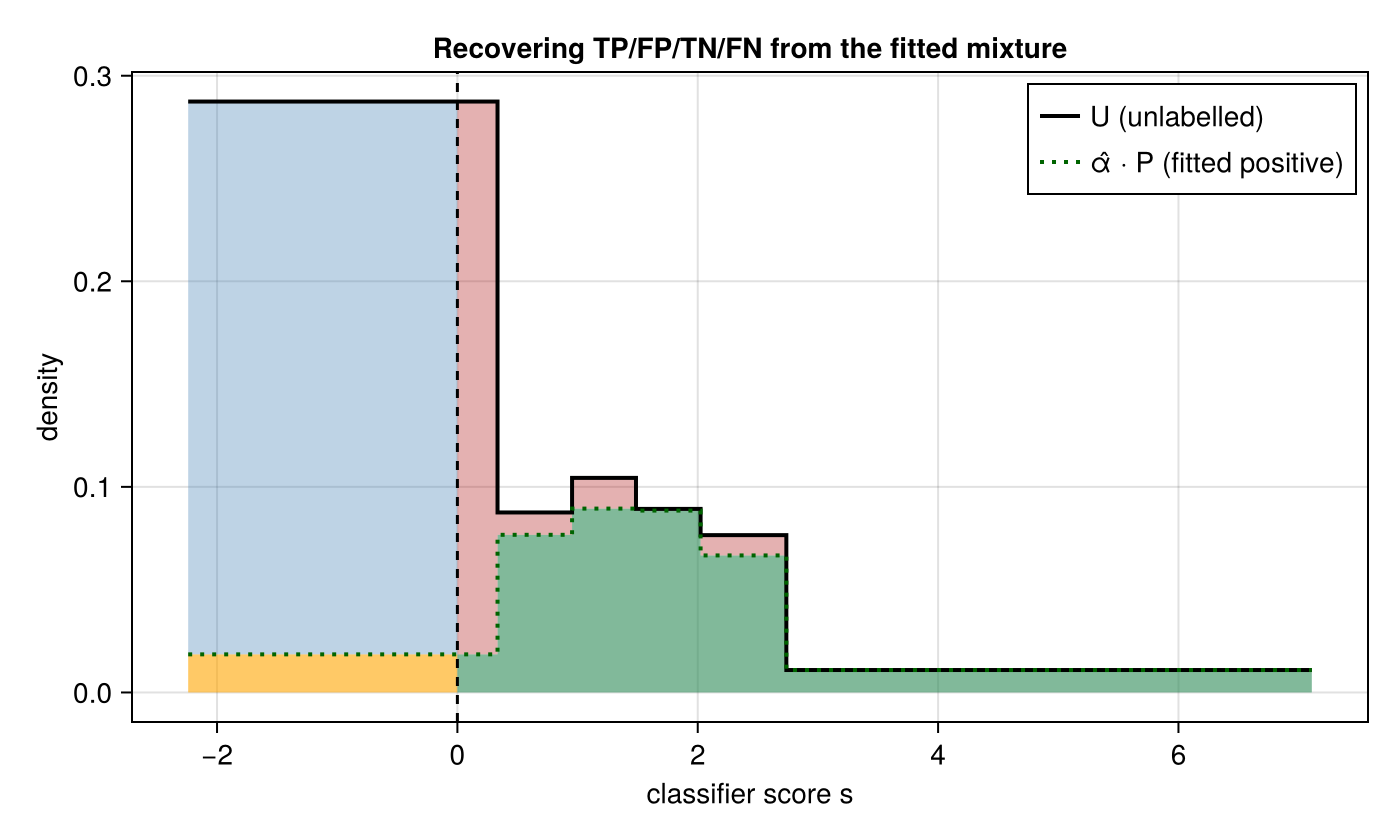
But that turns out to be enough. Jain, White & Radivojac 2017 points out that we actually only need to know the mixing proportion \(\alpha\) to be able to recover precision and recall. This surprising fact becomes obvious once you see the figure: each component of the confusion matrix is a clearly defined region that we can estimate empirically.
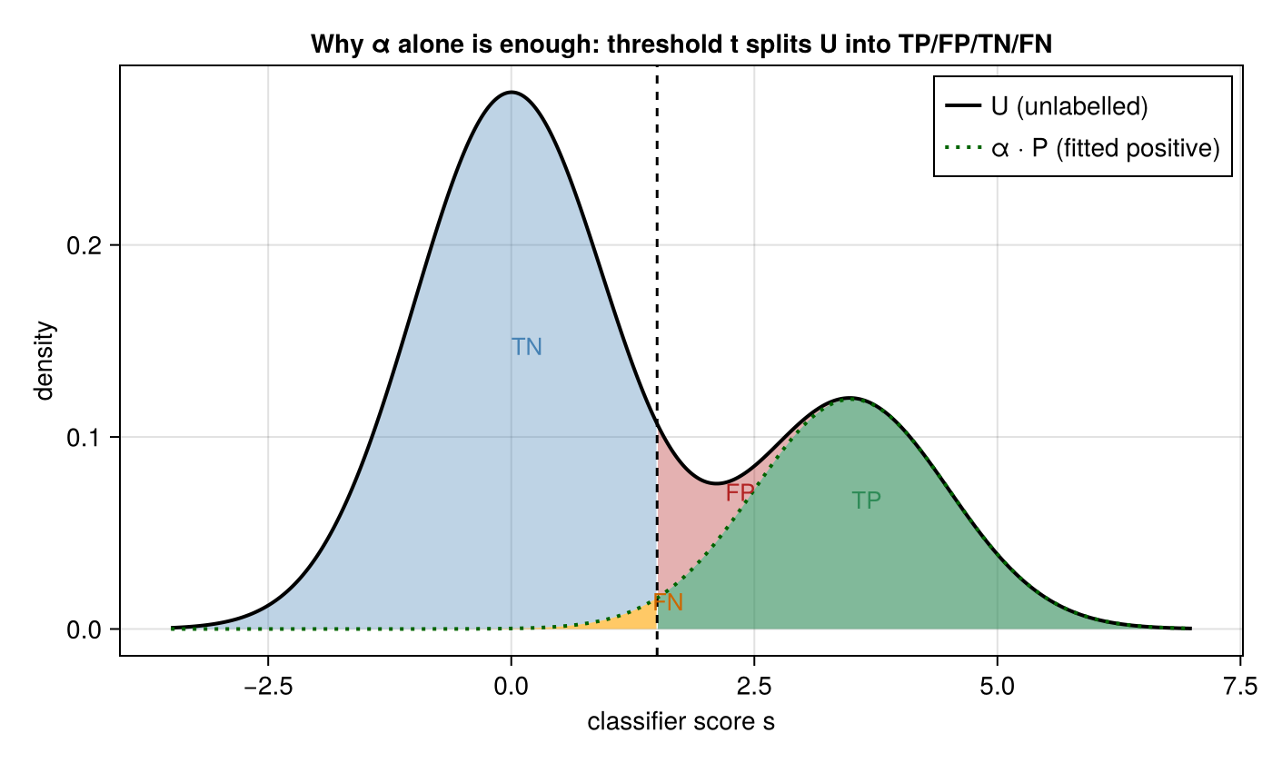
This hopefully holds at least approximately: like all classifiers, it should give us a region where precision is ≈ 100% (indeed we just need this region to be big enough).
Ok so how do we go about figuring out the positive mixing proportion \(\alpha\)?
Assumptions
For this we’re going to need slightly stronger assumptions than usual for positive unlabelled learning. Because we have a problem: we don’t have identifiablility between \(\alpha\) and \(N\). Consider the following animation of various decompositions of the same \(U\):
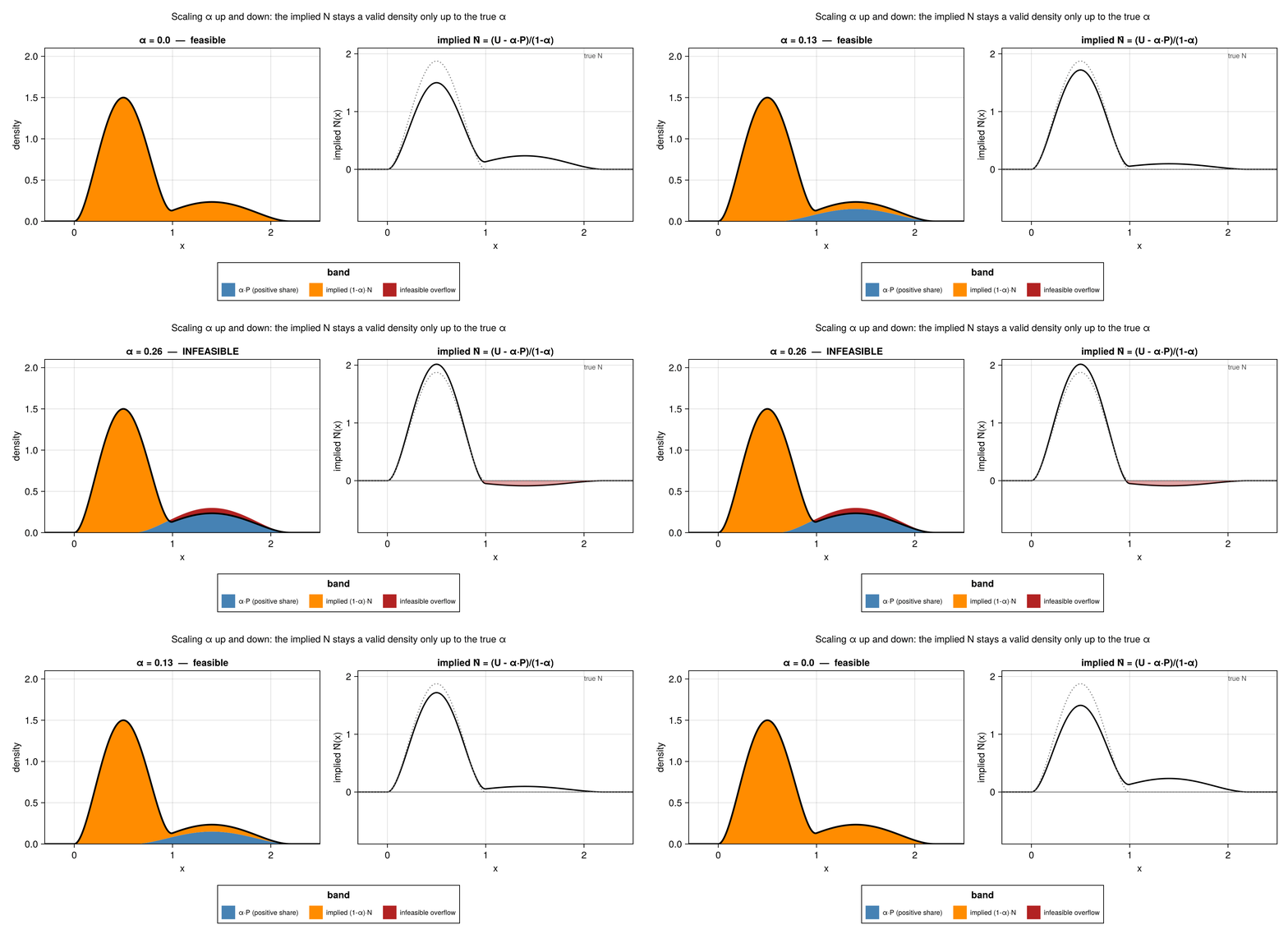
If the negative distribution overlaps with the positive distribution we can’t distinguish between the negative distribution having more overlap or \(\alpha\) just being smaller. To regain identifiability we’ll need to assume2 that there is no overlap: not everywhere, but for at least some region. If that holds then we know the biggest that \(\alpha\) can be and we’ll just use that \(\alpha\) as our estimate.
Density Estimation
This process suggests one approach to estimate \(\alpha\): we know the density of \(P\); we can scale it until just before we reach a contradiction where \(f(P) > f(U)\). We know that this has to happen in the region without overlap and precisely at the correct \(\alpha\) level!
But density estimation is scary: especially for complicated high-dimensional data like GenAI outputs. This would be hopeless: we have way higher dimension than we have sample sizes! But it would have been feasible if we had only a single dimension to work with…
The α*-trick
The classifier is a mapping from the complicated high-dimensional output space onto a convenient single dimension. Could we just use this distribution?
It turns out that we can though the justification is rather complicated (and doesn’t always hold!). Buckle up stats nerds while the others jump to the next section. Note I’ll be cribbing this from Lin and Long 2020
Fix the classifier score map \(C\) and write \(F, F_{P}, F_{N}\) for the CDFs of \(U, P, N\) in the original space, and \(G := C_{*}F\), \(G_{P} := C_{*}F_{P}\), \(G_{N} := C_{*}F_{N}\) for the induced CDFs of the score \(C(X)\). Call \(\gamma \in (0,1]\) feasible for a pair \((H, H_{P})\) if \((H - (1-\gamma)H_{P})/\gamma\) is itself a valid CDF Then
\[ \alpha_{0} := \inf\{\gamma \in (0,1] : \gamma \text{ feasible for } (F, F_{P})\}, \qquad \alpha^{*} := \inf\{\gamma \in (0,1] : \gamma \text{ feasible for } (G, G_{P})\}. \]
*$α^{} ≤ α0$, for any measurable \(C\).** Our induced classifier is a positive linear operators: if \(F - (1-\gamma)F_{P} \ge 0\) then \(C_{*}(F - (1-\gamma)F_{P}) = G - (1-\gamma)G_{P} \ge 0\) too. So every \(\gamma\) feasible in the original space stays feasible once we map \(X\) onto a single score; the feasible set can only grow, so its infimum can only shrink or stay put.
*$α^{} ≥ α0$, provided \(C\) is a strictly increasing transform of the true posterior \(P(Y{=}1 \mid X{=}x)\).** Suppose \(\gamma\) is infeasible for \((F, F_{P})\): there’s a set \(A\) with \(U(A) > 0\) where \((1-\gamma)f_{P}(x) > f_{U}(x)\), i.e. \(f_{P}(x)/f_{U}(x) > 1/(1-\gamma)\). Fit \(C\) to discriminate \(m\) labelled $P$-points from \(n\) unlabelled $U$-points, so \(\pi := m/(m+n)\) is its training prior; Bayes’ rule gives \(C(x) = \pi f_{P}(x) / (\pi f_{P}(x) + (1-\pi)f_{U}(x))\), so the inequality above is exactly \[ C(x) > t^{*} := \left(1 + (1-\gamma)\frac{1-\pi}{\pi}\right)^{-1}. \] Because \(C\) is monotone in the likelihood ratio, \(A\) maps onto exactly the super-level set \(\{c > t^{*}\}\) in score space, not merely into it, so the identical inequality \((1-\gamma)g_{P}( c) > g_{U}( c)\) holds on \(C(A)\), and \(\gamma\) is infeasible for \((G, G_{P})\) too.
Infeasibility in the one forces infeasibility in the other, so it’s subset giving \(\alpha^{*} \ge \alpha_{0}\).
Putting the two directions together: \(\alpha^{*} = \alpha_{0}\) whenever \(C\) is some strictly increasing function of the true posterior; it needn’t be the posterior itself. This disqualifies some classifiers such as SVMs whose margin has no general guarantee of approximating the posterior. But most things work at least approximately; and remember because we’re using an estimated \(C_{n}\) in place of \(C\), it only holds asymptotically3. But in practice it works pretty well.
Pulling it all together
Ok, so we have the classifier-induced distribution on positives, we have the classifier-induced distribution on unlabelled, now we just need to estimate \(\alpha\).
Remember we are trying to scale \(\alpha\) until we find a contradiction: thus we can summarize this as
\[ \max_{\alpha} \ \alpha \quad \text{subject to} \quad \alpha \, f_p^{(i)} \le f_u^{(i)}, \quad i = 1, \dots, B \]
where \(f_p^{(i)}\) and \(f_u^{(i)}\) are the heights of the $P$- and $U$-histograms on bin \(i\), out of \(B\) bins total. We use histograms as a convenient summary of the distribution to make things computationally easier.
We recognize this as a linear program! It’s pretty trivial to solve: \(\hat\alpha = \min_{i} f_u^{(i)} / f_p^{(i)}\) but let’s keep this formulation for now… we’ll see this pay off later on.
Real Example: Text Classification
First let’s show that this actually works using some real data: the Yahoo Answers Topic Classification Corpus (Zhang, Zhao & LeCun 2015, data).
These are about 1.4M yahoo answers split into 10 categories. We’ll fit a simple logistic regression on tf-idf features for the posts with Computers & Internet as our positive example. Then we’ll try to recover the classifier’s true performance with the only labelled data being positives from the test set.
Recovering \(\alpha\)
function histnd_density(scores::Tuple, edges::Tuple)
    d = length(scores)
    ns = ntuple(dim -> length(edges[dim]) - 1, d)
    widths = diff.(edges)
    counts = zeros(ns)
    for i in eachindex(scores[1])
        idx = ntuple(
            dim -> clamp(searchsortedlast(edges[dim], scores[dim][i]), 1, ns[dim]),
            d,
        )
        counts[idx...] += 1
    end
    bin_volume(idx) = prod(widths[dim][idx[dim]] for dim = 1:d)
    counts ./ (sum(counts) .* [bin_volume(idx.I) for idx in CartesianIndices(counts)])
end

# Quantile bins work better especially with sparse regions
function quantile_edges(vals::Vector{Float64}, nbins::Int)
    qs = range(0, 1, length = nbins + 1)
    edges = collect(quantile(vals, qs))
    edges[1] -= 1e-9
    edges[end] += 1e-9
    edges
end


function fit_alpha_lp(refs::Vector{<:Tuple}, mix::Tuple; nbins::Int = 6)
    k, d = length(refs), length(mix)
    # Bin edges come from the P sample(s) alone, not the pooled P+U sample: we
    # don't care about resolution in the region where only N has mass, since
    # the LP constraint there is slack no matter how it's binned.
    edges = ntuple(dim -> quantile_edges(vcat((r[dim] for r in refs)...), nbins), d)
    f_ref = [histnd_density(refs[i], edges) for i = 1:k]
    f_u = histnd_density(mix, edges)

    model = Model(HiGHS.Optimizer)
    set_silent(model)

    @variable(model, α[1:k] >= 0)
    @constraint(model, sum(α) <= 1)
    for cell in CartesianIndices(f_u)
        @constraint(model, sum(α[i] * f_ref[i][cell] for i = 1:k) <= f_u[cell])
    end

    @objective(model, Max, sum(α))

    optimize!(model)
    return value.(α)
end

score_x_U = logreg_score.(Ref(clf_x), U_docs)
alpha_hat_1 = fit_alpha_lp([(score_x_pref,)], (score_x_U,))[1]
t = 0.0   # the model's natural decision boundary: log-odds >= 0

# Split the mixture into the four quadrants a threshold cuts a fitted
# mixture into: recall (tpr) comes straight from the labelled reference
# sample; alpha_hat*n_u*tpr is the estimated TP count (the fitted
# positive curve, right of the threshold); whatever's flagged beyond
# that estimated TP count must be FP; the rest of the unlabelled pool
# splits into FN (missed true positives) and TN.
#
# Note recall = TP/(TP+FN) = (alpha_hat*n_u*tpr)/(alpha_hat*n_u*tpr +
# alpha_hat*n_u*(1-tpr)) = tpr exactly: alpha_hat cancels, so recall never
# actually needed the mixture-proportion estimate at all, only the labelled
# reference sample. Precision and FPR are the quantities alpha_hat buys you.
function quadrant_metrics(
    scores_pos_ref::Vector{Float64},
    scores_mix::Vector{Float64},
    alpha_hat::Float64,
    t::Float64,
)
    n_u = length(scores_mix)
    tpr = mean(scores_pos_ref .>= t)
    n_flagged = count(>=(t), scores_mix)
    TP = alpha_hat * n_u * tpr
    FN = alpha_hat * n_u * (1 - tpr)
    FP = max(n_flagged - TP, 0.0)
    TN = max(n_u - n_flagged - FN, 0.0)
    (precision = TP / (TP + FP), recall = TP / (TP + FN), fpr = FP / (FP + TN))
end
| Quantity | Value |
|---|---|
| True alpha | 0.3 |
| Recovered alpha (PU estimate) | 0.286 |
| 95% bootstrap CI | [0.231, 0.305] |
Recovering Precision and Recall
| Quantity | Recovered (PU estimate) | 95% CI | Oracle (true labels) |
|---|---|---|---|
| Prevalence (α) | 0.286 | [0.231, 0.305] | 0.3 |
| Recall (TPR) | 0.892 | [0.877, 0.906] | 0.893 |
| Precision | 0.896 | [0.737, 0.941] | 0.942 |
| FPR | 0.041 | [0.024, 0.099] | 0.024 |
We see that we fairly closely recover recall. This is not suprising as it’s basically free. Precision and FPR however depend on the prevalence and we get close but we’re a little low.
How Many Bins?
extra_ref = x_unlab[5000:7999]
extra_pos = x_unlab[8000:10999]
x_ref_big = vcat(x_ref, extra_ref)

n_pos_U_big = n_pos_U + length(extra_pos)
n_neg_U_big = round(Int, n_pos_U_big * (1 - true_alpha1) / true_alpha1)
U_pos_big = vcat(x_unlab[1:n_pos_U], extra_pos)
U_neg_big = neg_pool[10000:(9999+n_neg_U_big)]
U_docs_big = vcat(U_pos_big, U_neg_big)

score_x_pref_big = logreg_score.(Ref(clf_x), x_ref_big)
score_x_U_big = logreg_score.(Ref(clf_x), U_docs_big)

# A third, much bigger tier — using almost all of the PC-flavored and
# background docs that "small"/"big" leave untouched (see the BG_CAP
# comment in Loading the Data: most of what gets cleaned there never
# gets used downstream) — to see the bias-variance tradeoff actually
# resolve at scale, not just the 2.5x jump "small" -> "big" gives us.
huge_ref = x_unlab[11000:20999]
huge_pos = x_unlab[21000:end]
x_ref_huge = vcat(x_ref_big, huge_ref)

n_pos_U_huge = n_pos_U_big + length(huge_pos)
n_neg_U_huge = round(Int, n_pos_U_huge * (1 - true_alpha1) / true_alpha1)
U_pos_huge = vcat(U_pos_big, huge_pos)
U_neg_huge = neg_pool[(9999+n_neg_U_big+1):(9999+n_neg_U_big+n_neg_U_huge)]
U_docs_huge = vcat(U_pos_huge, U_neg_huge)

score_x_pref_huge = logreg_score.(Ref(clf_x), x_ref_huge)
score_x_U_huge = logreg_score.(Ref(clf_x), U_docs_huge)

nbins_sweep = [4, 6, 10, 15, 20, 30, 50, 80]
sweep_small =
    [fit_alpha_lp([(score_x_pref,)], (score_x_U,); nbins = b)[1] for b in nbins_sweep]
sweep_big = [
    fit_alpha_lp([(score_x_pref_big,)], (score_x_U_big,); nbins = b)[1] for b in nbins_sweep
]
sweep_huge = [
    fit_alpha_lp([(score_x_pref_huge,)], (score_x_U_huge,); nbins = b)[1] for
    b in nbins_sweep
]
You might be curious why we have only 6 bins before? Like surely we want to have better representation of the distribution than this coarse binning allows?
It turns out that we don’t: there’s a bias variance tradeoff involved. Holding the data fixed we can see that our estimates degrade as we increase the number of bins to 30.
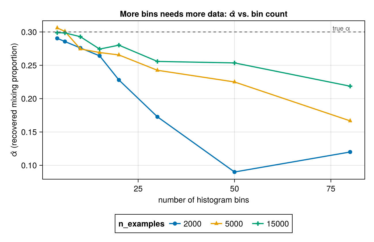
Funnily enough this is a variance problem that turns into a bias problem! As we add bins each bin’s sample size decreases and thus the density estimate gets noisier as bins get finer and finer. They do remain unbiased though: this is only a variance problem.
But remember that our \(\hat\alpha\) is the max over the per-bin constraints. Thus we’re picking from the tail of the distribution which only gets worse when we have higher variance and it only gets worse by underestimating \(\alpha\).
We can see this by increasing the size of the test set.
Why: Variance Becomes Bias
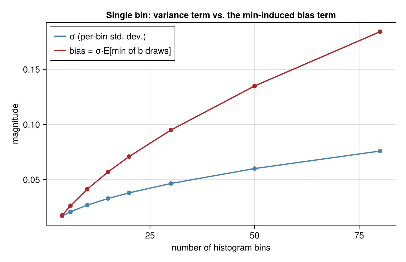
Our \(\hat{\alpha}\) is the minimnum over bins. While a single bin’s ratio estimate has variance that shrinks with more data and grows with more bins, because we take the minimum over these that symmetric noise turns into a chronic underestimation bias: the more bins we have the more changtes that a single unlucky low draw gets picked.
Complications
The natural question is how can you be sure that the positive distributions match? For instance, suppose we want to count another class as positives. You can do the same thing as before but now you have a problem: you have positive distributions for both and you know the real positive class is a mixture of the two: you just have no way of knowing the mixing weights!
To my knowledge I haven’t seen this addressed in the literature. Indeed this linear program formulation hasn’t really showed up: this is a little twist of mine. But it’s about to pay off because it suggests a straightforward extension: just add this to the mixture model problem! Now instead of a single distribution you have multiple:
\[ U = \sum_{i} \alpha_{i} P_{i} + N \]
and so our linear program now is just to find the solution to
\[ \max_{\alpha} \sum_{i} \alpha_{i} \quad \text{s.t.} \quad \forall \text{ bins } j : \sum_{i} \alpha_{i} f_{i}(p_{j}) \le f(u_{j}) \]
To break this we need to add more constraints! Notice that we can also add other distributions; so what if we had a classifier for each individual positive class in addition to the combined classifier. This would give us three sets of constraints:
\[ U_{k} = \sum_{i} \alpha_{i} P_{i,k} + N_{k} \]
\[ \max_{\alpha} \sum_{i} \alpha_{i} \quad \text{s.t.} \quad \forall k, \text{ bins } j : \sum_{i} \alpha_{i} f_{i,k}(p_{j}) \le f_{k}(u_{j}) \]
Multiple classifiers on the Data
Let’s see this in practice!
Let’s look at some closely related catgories Education and Family.
We note that the identifiability problem is real here.
| Quantity | Recovered (PU estimate) | 95% CI | Oracle (true labels) |
|---|---|---|---|
| Recall (TPR) | 0.808 | [0.781, 0.828] | 0.836 |
| Precision | 0.752 | [0.654, 0.829] | 0.762 |
| FPR | 0.421 | [0.331, 0.505] | 0.392 |
Now we see that we can easily distinguish between the two!
Conclusion
I was surprised when I found out that even in this initially hopeless setting you can still recover performance. Now, your assumptions are fragile, but you indeed can measure what you can’t label!
As we get deeper into the generative AI era methods like these start becoming more interesting. Synthetic data for training and evaluation are hot topics. Doing it in a statistically robust manner is a space for statisticians to contribute!
-
Bekker and Davis 2020 has an excellent survey for folks who want to dig in deeper ↩︎
-
And this is really an assumption: we cannot falsify this assumption without access to true labels ↩︎
-
You also need to do some sample splitting too ↩︎