Up until this week I had never used feature importance. I roughly knew that it existed and had no inkling of the particulars. This was fine; I had never had a compelling answer to the “so what” question: what would I do differently once I got the results?
Thus I really only looked into it after a work situation compelled me to calculate it. And what I found was disappointing: while the method seems perfectly reasonable on toy examples with independent features, once you start introducing dependence (i.e. most real datasets) you can get wildly varying results.
How Permutation Feature Importance Works
At first, the logic of feature importance is seductive. A feature is important to a model if without it the model is less accurate. A feature is not important if the model does just fine without it.
The obvious approach is an ablation study: simply remove the feature, retrain the model, and calculate how much the loss went up:
\[ VI_{k} = \frac{1}{n} \sum_{i} L(y_{i}, f_{-k}(x_{i,-k})) - \frac{1}{n} \sum_{i} L(y_{i}, f(x_{i})) \]
where \(f\) is our fitted model and \(f_{-k}\) is the model retrained without feature \(k\). If the loss jumps once the feature is gone, the feature was important.
But ablations are really expensive: when it takes a day to fit a neural network, do you really want to train a new one for each feature?
So we need something cheaper. Enter permutations.
It seems like the origin of this method is Breiman’s Random Forest paper where out-of-sample data is permuted and sent down the regression trees. We can generalize this a little more and use any sort of out-of-sample data and permutations. Instead of retraining, we keep the original model and feed it \(x_{i, \pi(k)}\): the $i$-th row with feature \(k\) replaced by its value from a permuted row.
\[ VI_{k}^{\pi} = \frac{1}{n} \sum_{i} L(y_{i}, f(x_{i, \pi(k)})) - \frac{1}{n} \sum_{i} L(y_{i}, f(x_{i})) \]
And we probably repeat this a few times to average out over the random permutation.
In code:
using Random, Statistics

function permutation_importance(predict, xs, ys; nrep = 10)
    loss = mean((predict(xs) .- ys) .^ 2)

    importances = zeros(size(xs, 2))

    for k in axes(xs, 2), _ = 1:nrep
        xs_permuted = copy(xs)
        xs_permuted[:, k] = xs_permuted[randperm(size(xs, 1)), k]
        permuted_loss = mean((predict(xs_permuted) .- ys) .^ 2)
        importances[k] += (permuted_loss - loss) / nrep
    end

    return importances
end
This doesn’t seem to be intended as more than a heuristic: Breiman writes “A start on this problem [of feature importance] is made by using internal out-of-bag estimates, and verification by reruns using only selected variables”. But that caveat doesn’t seem to have stuck and you can google “permutation feature importance” to see all the places that more or less accept this as standard practice.
Where it goes wrong
As you do your Google search, however, you’ll start to see warning signs. For instance the scikit-learn documentation has a very prominent warning:
Features that are deemed of low importance for a bad model (low cross-validation score) could be very important for a good model. Therefore it is always important to evaluate the predictive power of a model using a held-out set (or better with cross-validation) prior to computing importances. Permutation importance does not reflect the intrinsic predictive value of a feature by itself but how important this feature is for a particular model.
This is a useful note for any notion of importance. I’d go a little further than them and note that importance is tied not only to a particular model but also a particular dataset! For instance, gender may be an important variable for a model on the general population, but if you restrict your data to a single gender then it’s clearly unimportant (and permutations will bear that out as nothing will change). Good stuff with lots of bolding and flagging.
What is less emphasized is a section towards the end on “misleading values on strongly correlated features”. It’s quite easy to skip. They state:
When two features are correlated and one of the features is permuted, the model still has access to the latter through its correlated feature. This results in a lower reported importance value for both features, though they might actually be important.
It’s not entirely clear to me that this is a problem: recall that we were previously thinking of ablation studies. If we had done such a study we would actually find that the importances of the correlated features are basically zero: the model still has access to the correlated feature and can easily adapt. So this is the correct answer for individual feature importances and not a problem.
Really, the scary thing would be if we could manufacture feature importance for features that aren’t at all important. So let’s make that happen.
Checkerboard Simulation
Consider a checkerboard pattern: the target is \(y = \text{sign}(x_{1} x_{2})\), so it’s \(+1\) on the diagonal quadrants and \(-1\) on the off-diagonal ones. Our data lives almost entirely on the diagonal quadrants, so \(y = +1\) for every point we’ll ever collect. Then we add just two outliers the off-diagonal squares.
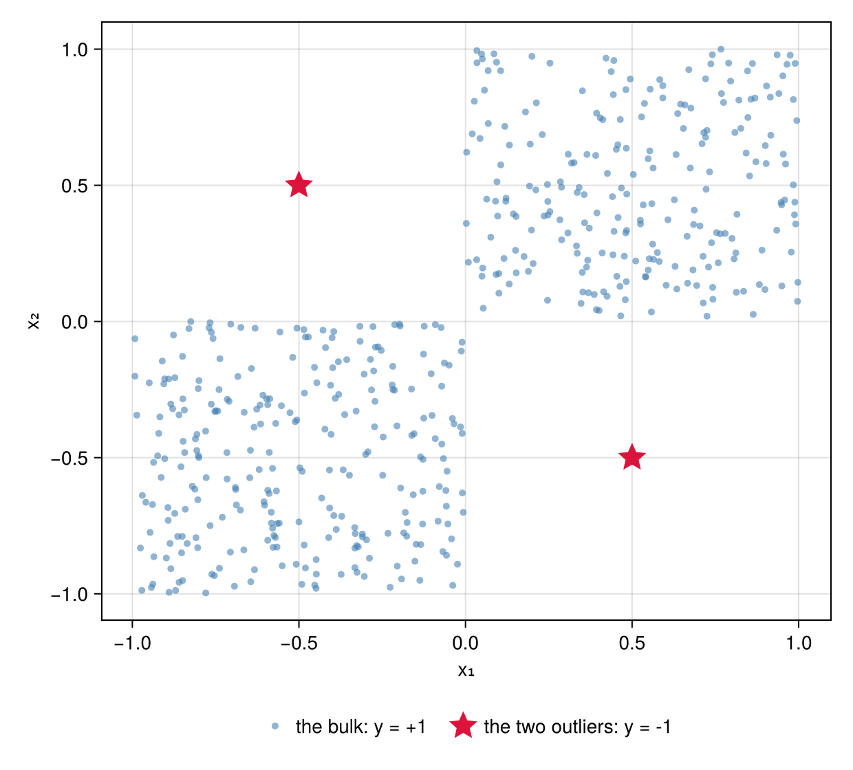
Figure 1: The training data: the bulk lives on the diagonal quadrants where y = +1; the two outliers sit alone in the off-diagonal quadrants.
Now consider a 1-nearest neigbhor model
function knn1(xtrain, ytrain)
    function predict(xs)
        map(axes(xs, 1)) do i
            dists = [
                sum(k -> (xtrain[j, k] - xs[i, k])^2, axes(xs, 2)) for j in axes(xtrain, 1)
            ]
            ytrain[argmin(dists)]
        end
    end
end
On fresh data from the same distribution, this model is essentially perfect: new points land in the diagonal quadrants next to training points that all say \(+1\). Baseline loss ≈ 0. The two outliers don’t matter at all: they are beaten out in any region with actual data.
But now permute a feature. Shuffling \(x_{2}\) breaks the link with \(x_{1}\), so half the sample lands in the off-diagonal quadrants where the nearest neighboors are the outliers.
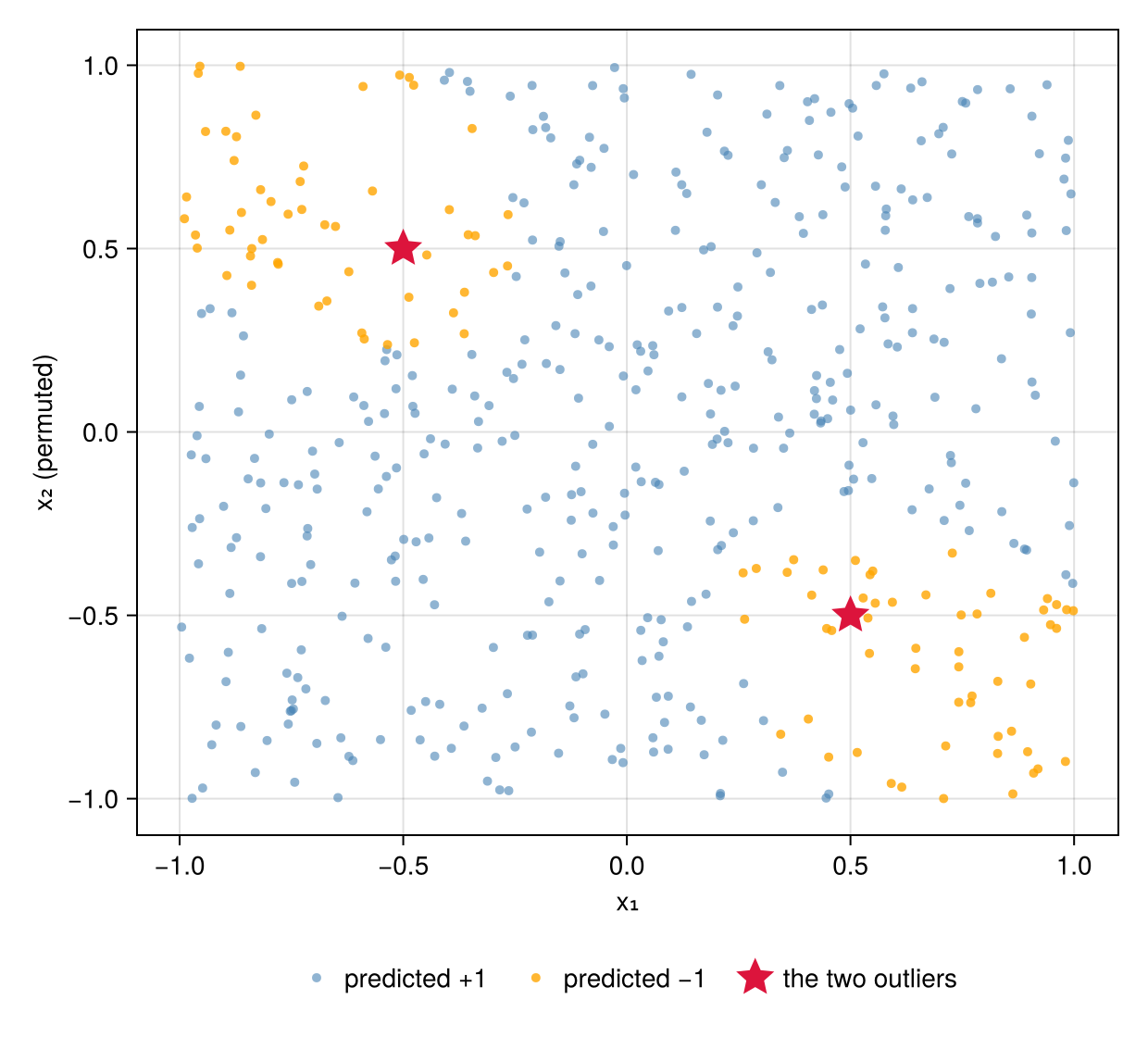
Figure 2: The test set after permuting x2 (outliers labeled -1 here). Half the sample now sits in the same quadrant as the outliers
Every true label is \(+1\), but the predictions for the permuted points come straight from the two outliers. So the entire permutation importance is determined by their two labels:
- both \(+1\)
- the off-diagonal predictions happen to be right, the loss doesn’t move, and both features are reported unimportant.
- one of each
- half the off-diagonal predictions are wrong and both features get a middling importance.
- both \(-1\)
- the off-diagonal predictions are all wrong and both features are reported as hugely important.
Noticeably, this doesn’t change with more data! No matter how many bulk data points we add, the off-diagonal quadrants stay empty, the outliers keep their monopoly on them, and the importance stays pinned wherever those two labels put it:
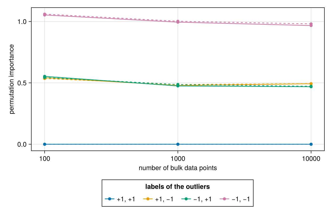
Figure 3: Permutation importance of x1 (solid) and x2 (dashed) as the bulk data grows, for each labeling of the two outliers. The curves are flat: the two points decide the importance while becoming increasingly minute proportions of the data.
So whether these features look unimportant, middling, or critical comes down to two data points that can constitute an arbitrarily small proportion of the data. And note that the ablation answer here is unambiguous: drop either feature and retrain, and the model still predicts \(+1\) wherever the data lives. Ablation importance is thus zero: permutation importance is inventing importance out of nothing.
It’s not just nearest neighbors
Consider duplicated features: let \(x_{2}\) be an exact copy of \(x_{1}\) and let \(y = x_{1}^{2}\). Then these three models are completely equivalent on the diagonal support.
n = 100_000
x1 = rand(n) .* 2 .- 1
xs_dup = hcat(x1, x1)          # x₂ is a copy of x₁
ys_dup = x1 .^ 2

models = [
    "f(x) = x₁²" => xs -> xs[:, 1] .^ 2,
    "f(x) = x₁x₂" => xs -> xs[:, 1] .* xs[:, 2],
    "f(x) = x₂²" => xs -> xs[:, 2] .^ 2,
]
Thus we get the same predictions and the same (zero) loss. But while these models are otherwise indistinguishable by any amount of data, we find that they have wildly different permutation importances.
| Model | Importance of x₁ | Importance of x₂ |
|---|---|---|
| f(x) = x₁² | 0.18 | 0.00 |
| f(x) = x₁x₂ | 0.31 | 0.31 |
| f(x) = x₂² | 0.00 | 0.18 |
Which feature is “important” is entirely determined by which representation your fitting procedure happened to land on: whether it used \(x_{1}\), the interaction, or \(x_{2}\). You can see why when we plot what these models do in the off-diagonals.
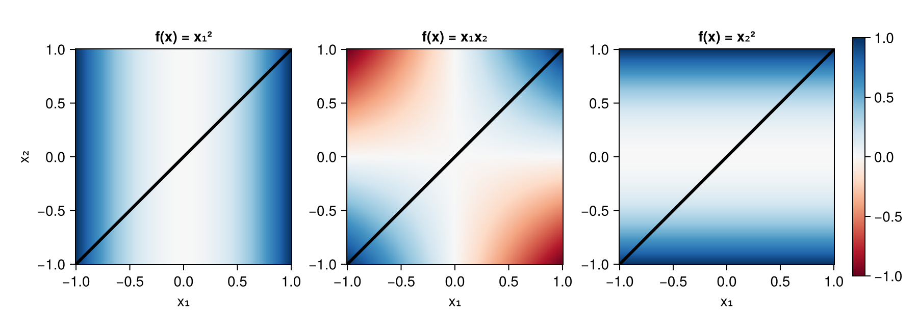
Figure 4: Three models that agree exactly on the data (the black line, (x_{2} = x_{1})) and nowhere else. Permutation importance forces them to extrapolate into regions with no support.
The problem in both examples is that permutation breaks any dependence1 between our variables. Thus we end up evaluating the model in regions where the original data has little to no support. Nothing constrained the model in these regions, so its extrapolations can be arbitrarily bad and permutation makes these regions influential. We’re no longer measuring the contribution of a feature: we’re just measuring what the model extrapolates.
You don’t even need pairwise dependence to trigger this. Let \(x_{1}\) and \(x_{2}\) be independent coin flips and set \(x_{3} = x_{1} x_{2}\): every pair of features is independent, yet permuting any one of them still pushes you outside the support. This same parity construction works in any dimension resulting in every proper subset of the features jointly independent while the whole is dependent.
What to do instead
I’m hardly the first person to point this out: Hooker, Mentch, and Zhou (2021) is a great review of this problem. Amusingly, the paper’s original title was “Please Stop Permuting Features: An Explanation and Alternatives”.
They diagnose the dependence problem with a more subdued example, but it’s effectively the same problem. They have an elegant analysis showing that several methods converge to the results you’d get if you ablated features and retrained:
- Conditional Variable Importance
- instead of permuting, you fit the conditional distribution \(x_{k} \mid x_{-k}\) and sample replacement values from it, so the “shuffled” data stays on the support.
- Permute and Relearn Importance
- you permute the feature and retrain the model on the permuted data.
- Condition and Relearn Importance
- you do the conditioning as above and also retrain.
But, um, all of these methods are basically refitting the model or estimating complicated conditional distributions, so you might as well do the ablation at that point.
Does any of this matter?
Before you make your GPU go brrr running some ablations, let’s come back to the “so what” question. What’s the point of this exercise? What are we to do with a variable that has low, medium, or high importance?
Think of the things you can do to a variable:
- If I dropped this variable what happens?
- If I improved my measurement of this variable what happens?
- If I intervened on this variable what happens?
- If I had a different distribution of this variable what happens?
Only the first is answerable by ablation. And even then with modern approaches, it’s not the worst thing in the world to just keep variables around. The rest are not well addressed by ablation, instead you should consider measurement error models, causal inference, and distribution shift.
I started looking into permutation importance mostly because someone asked for it. I confronted them with the “so what” question: this is good practice to avoid the XY problem where you end up addressing a superficial question X instead of the root problem Y. Sure enough, the real reason was that they wanted an intuitive explanation for the model. Which is definitely not helped by feature importances either. So I’m still bereft of a compelling reason to use feature importances.
-
Note it’s really dependence, not strictly correlation, that causes this: we can replicate the problem with zero correlation by rotating the checkerboard example 45° to form an X pattern. ↩︎