Today was a big payoff for my employers. Not that the other days weren’t helpful, but I found several new ideas that I’d like to try on some of our problems. Going to these conferences is always helpful: for instance I picked up PPI from a conference at Stanford right when the paper came out. I ran into my advisor yesterday and she was bewildered by the wide array of sessions I was attending (aka why do you care about spatial statistics and also surveys?). The academic path requires specialization but for industry it pays to be a generalist and take the best from everywhere.
AI, LLMs, Machine Learning, and Survey Research
Lots of talks in this session so each was just a brief hit. Coming from industry this was awesome as it got me exposure to a lot of ideas quickly and I can follow up as needed.
-
Brisilda Ndreka started off discussing influence in social networks. The issue is that influence is hard to estimate: homophily (you make friends with those you’re similar to) and contagion (you make your friends more similar to you) are confounded. I’ve always had a hard time explaining this to folks: she has a figure I think makes it clear
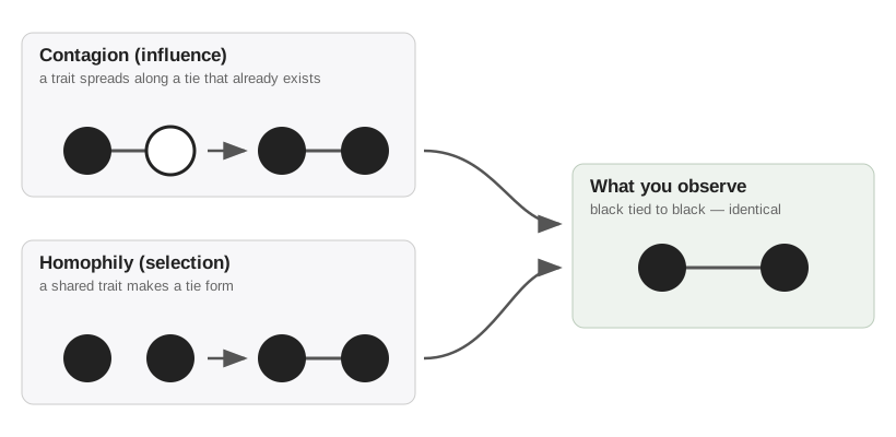
Figure 1: Homophily and contagion are confounded: two different mechanisms produce the same observed black-tied-to-black pattern. In contagion a trait spreads along a tie that already exists; in homophily a shared trait is what makes the tie form. The observed data at the end is identical either way: we can’t distinguish.
The way out is to get at the unobserved trait driving the homophily: if you could actually measure “who is similar to whom” you’d just control for it and whatever influence is left over is contagion. That’s an omitted-variable-bias problem, so the fix is to recover a proxy for the missing variable. So you use network-embedding methods to embed each person into a latent social space (a handful of coordinates summarizing their position in the friendship graph) and then you adjust for those coordinates the way you would any other confounder. She backed this up with a simulation study pitting latent space, SDNE, a latent factor model, and Node2Vec against each other, with the latent space approach coming out on top.
-
Asha Pantula presented feature selection for scalar on function regression. Another instance of a MIP problem for best-subset selection: apparently this is growing due to the computational advance.
-
Brandon Sepulvado and Sophie Hensgen both presented talks on integrating synthetic respondents for surveys. The common result was that LLMs aren’t very accurate for individual results but can replicate overall totals somewhat, though the variance is too small. Interestingly it was suggested that this is more true for studies which are plausibly in the training sets: it’d be wild if these results are basically just artifacts of the LLM regurgitating studies (makes the lack of individual correlation make sense). They found that adding more information to the LLM’s context improved results: give the model previous responses from the human and it’s easier to predict the new response (reasonable though I wonder if you’re better off with a non-LLM model at that point). And of course PPI gets used heavily. You might wonder why bother with synthetic respondents? Mostly because you can throw a ton of questions at them and they don’t get mad. In particular factorial survey experiments where you send surveys with multiple settings are an interesting application: basically you ask a ton of variants of “A {year} year old {man/woman} works as a {profession}: is {salary} a fair wage?” and then you can learn something about the surface of opinions.
-
Mi Huynh investigated whether LLM translations of survey questions were up to snuff. And like most LLM-things: sorta but not perfectly enough to really want to use it on anything important.
-
Noah Bassel presented on ML for nonresponse bias. You can target likely responders and create a class where all units have the same probability of response (called “class-based non-response weighting”). The pitch was to use ML rather than the usual grouped categorical variables plus raking.
-
Moinak Bhaduri looked into modeling respondent uncertainty. Basically letting a Likert-scale response be genuinely indecisive, modelling it as a mixture between a multinomial and a uniform distribution (indecisive).
Bayesian Approaches for Complex Problems in Causal Inference
Michael Daniels started us off with a Bayesian non-parametric approach for semi-competing risks. I found this fascinating; competing risks are things like causes of death: you either die of cancer or you die of a car crash, you can’t do both. This has implications for studies of things like cancer survival rates: the car crash censors your survival time due to cancer. Semi-competing risks are not symmetric: consider a disease relapse and death. Death prevents you from ever relapsing, but relapsing doesn’t prevent you from later dying: thus one-way competition.
Censoring (and errors in measurement) in general is such a pain to work with frequentist techniques. Bayesian approaches though are sweet: you basically just write out a process for corrupting the true latent data and then it’s just MCMC again. Of course you need some assumptions, but nicely you can structure the priors as a d-vine to get a mix of identifiable distributions separated from the non-identifiable distributions. Then you use non-parametrics for the observables and semi-parametrics with wide priors for the parts where we don’t have any information.
Nathan Wikle considered the problem of attributing pollution to CAFOs (basically pig farms). The idea being that the effects should be pretty local but also there might be a number of sources and other confounders around which could explain away any particular farm’s impact. The estimand question was interesting: you only get one realization of the world, so is the estimand the point process itself or an average marginalized effect over a fixed set of interventions? Of course imposing structure to answer that question is easier in a Bayesian setting.
Antonio Linero gave a talk on subgroup selection. CATEs are hard to estimate: you might just want to get your policy right and call it a day. But there’s an issue: if you just look at which groups benefit from treatment you suffer from winner’s curse. Like there’s always going to be a group that “benefitted” in the data unless there’s a tie. But if there’s no real effect (or a small effect) that could just be noise and you’re too optimistic about what groups to pick.
What you want instead is something that will generalize well so add a penalized norm for prediction error:
\[\sum (\hat{\pi}(x_{g}) - \pi(x_{g}))^{2} + \lambda \sum_{g} \lVert \hat{\pi}(x_{g}) - \bar{\pi}_{g} \rVert^{2}\]
Indeed they show that set \(\lambda=0\) (ignoring the generalization) this is actually risk-seeking: you’re going to slice your data thinner and thinner because you’re incentivized to find small subgroups which are wildly poorly estimated because that’s how you get the largest gaps. You lean even harder into the winner’s curse. They show that for λ=1 this actually simplifies to a CART model fit on the CATE (though not to optimality).
Harnessing Artificial Intelligence for Causal Inference and Experimental Design
Simon Mak discussed digital twins: these are computer simulations which are a proxy for the real world. But they’re often way too expensive to experiment with so you need a surrogate model for your simulation. In this case they were working on a rover for which they had a simulator and were trying to find the best path over some complicated terrain. Their surrogate is the ever popular Gaussian process.
They parametrized their path-finding with a series of binary features and fit the surrogate using the kernel \(\exp(-\sum\theta_{i} I(x_{l} \ne x_{r}))\). The benefit of the GP is that it’s quite flexible and also has natural sequential exploration.
They call their method QuIP and it does Hamming-optimal design. This is an assignment problem that can be efficiently solved as a MIP (again!).
Susan Murphy then discussed RL for digital health interventions: they have a caregiver and child pair and want to motivate them to keep taking medication. The RL algorithm decides whether to send them notifications or ask them to participate in certain games and exercises designed to improve compliance. But of course that’s a burden so you don’t want to send too many otherwise you end up burning them out. This naturally leads to a DAG and, of course, you want the RL algorithm to learn the correct causal effects to be able to intervene optimally. This is particularly hard because the negative burden is immediate while the other interventions act on the scale of weeks and have impact into the future.
Dylan Small’s talk never discussed LLMs but I cannot fathom why not. The problem was the idea of pre-registration. Observational studies are hard and you want to be able to look at the data and try to figure out what sort of biases you need to correct for. Unfortunately that biases your results: especially if you really want some outcome to occur. Thus pre-registration saves you from yourself but also binds you too tightly to make needed adjustments.
The idea then is the two-team cross study. One team will do EDA on one half of the dataset and the other team will do the same on the other. They’ll write out an analysis plan and then swap and execute the others’ plan on their original data. Because there’s two teams there’s no overlap: nobody has to worry that somehow subconsciously they made decisions about the forbidden half of the data.
This is expensive: you need a ton of folks. Thus it’s not clear why you don’t just have LLMs do it! You can provide a ton of prompting and the sorts of things that one should consider and let the LLMs go on their side of the data. Naturally the answer is probably they’re not good enough yet, but I’d have expected to at least try it out.