I was listening to a lovely podcast with Ada Palmer on Machiavelli1 when I got nerdsniped by a problem posed by a Jane Street interstitial ad:
@46:35 Here you’ve got an image dataset, but half of the images in it have been corrupted. They’ve been scrambled in a consistent way. Like, if the pixel on the top right got swapped with the pixel in the middle, the same swap happened for all of the images in the second half of the dataset.
Identifying the Corrupted Images
The first thing to note is that this is hopeless if the images are static noise: you couldn’t tell one from the other. This suggests that the distinguishing feature between a permuted image and an uncorrupted one is structure!
One sort of structure2 is local consistency: we expect neighboring pixels to have similar values. We can quantify this by the average deviance from a smoothed version of the image
\[ \delta = \frac{1}{N}\sum_{i,j} (X[i,j] - S[i,j])^{2} \]
where \(S[i,j]\) is the smoothed version. All things being equal we should see smaller values for originals and larger for permuted images.
However this isn’t sufficient because different images have different baseline values. An image of the ocean and sky with varying shades of blue will likely have a smaller value than a kaleidoscopic picture of confetti. So we don’t want to set a threshold on δ itself.
But suppose we had a new permutation and calculated:
\[ \Delta = \delta(\text{new permutation}) / \delta(\text{original})\]
For uncorrupted images this will catastrophically disrupt the structure and we’ll see a jump in deviances so \(\Delta \gg 1\). But for an already-permuted image it won’t make a ton of difference; it’s just a different random permutation and thus \(\Delta \approx 1\). Thus we can set a threshold on \(\Delta\) and separate the images.
Testing on Real Data
We can empirically test this using the CIFAR-10 dataset of natural 32×32 images. We’ll transform this into grayscale to remove a little more information but also make the math cleaner (we can easily formulate multivariate versions).
using Random, Statistics, LinearAlgebra
using MLDatasets
using ImageFiltering
using DataFrames
using Graphs
using AlgebraOfGraphics, CairoMakie
using GraphMakie, NetworkLayout

Random.seed!(1234)

features = CIFAR10(:train).features
W, H = size(features, 1), size(features, 2)
NPIX = W * H

N = 2000
luma =
    0.299f0 .* features[:, :, 1, 1:N] .+ 0.587f0 .* features[:, :, 2, 1:N] .+
    0.114f0 .* features[:, :, 3, 1:N]

images = [Float64.(luma[:, :, k]) for k = 1:N]
We can easily construct our two measures using a convolution kernel.
function δ(image)
    smoothed = imfilter(image, ImageFiltering.centered(ones(3, 3) ./ 9))
    return mean((image .- smoothed) .^ 2)
end

function Δ(image)
    permuted = reshape(vec(image)[randperm(length(image))], size(image))
    return δ(permuted) / δ(image)
end
To test, we draw a single shared permutation, apply it to a random half of the images (the “corrupted” set), and leave the rest alone. Then we score every image with both δ and Δ.
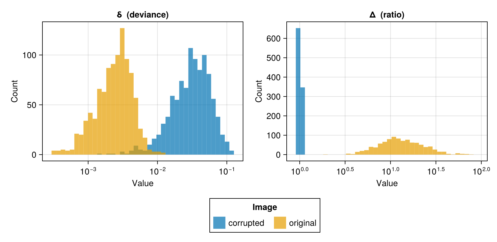
Figure 1: Histograms of (delta) and (Delta): we see that we can achieve good separation with (delta) but perfect separation with (Delta).
The two populations come apart more or less cleanly: originals sit at small δ and large Δ, corrupted images at large δ and \(\Delta \approx 1\). Note that we see a decent bit of overlap in δ-space while a threshold on Δ cleanly separates the two distributions.
You might worry that we could accidentally pull the identity permutation or a flip or rotation which preserves the local information. While quite rare you can guard against this by turning this procedure into a formal permutation test and calculate \(\delta\) for a larger number of permutations. You can then set the Type I error rate pretty low as your Type II error rate remains quite low given the stark gap in the \(\Delta\) distributions.
Recovering the Permutation
This has already been quite a fun problem, but I think we can go further. Now that we have identified the corrupted images, let’s see if we can reverse the permutation!
On the face of it this is an intimidating task: there’s a ridiculously huge space of possible permutations (1024! has a lot of digits) so we have to be judicious in our search. To add to the difficulty, note that if we only had a single image we again wouldn’t be able to do this: multiple real images could just be different permutations of the same pixels.
The only thing that saves us is that the corrupted images share the same permutation, so we can use our assumption of local consistency again.
We calculate the correlation across images of each pixel with each other pixel. Nearby pixels should be highly correlated and far-away pixels should not. Thus we should be able to identify each pixel’s neighbors even after permutation (though they’ll of course be scattered).
You can see precisely this in the animation below: on the left are the unaltered images, on the right the permuted ones. We iterate through the “active” pixel (marked in black) and draw a heatmap of every other pixel’s correlation with it. On the left the high-correlation pixels cluster tightly around the active point; on the right the same set of neighbors light up but are scattered across the image. There are some longer range correlations especially around the edges but the strongest remain quite close by.
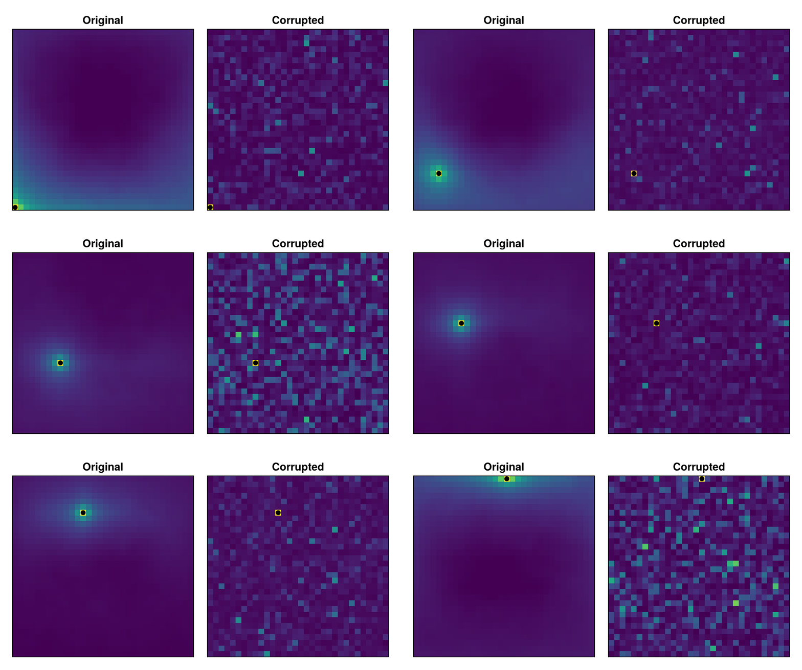
Figure 2: Correlation heatmaps: the left shows nearby pixels are highly correlated with the target. These same pixels light up for the corrupted data but are scattered.
We can use these correlations to try and reconstruct the neighbor graph. We’ll have each pixel nominate its 8 most-correlated partners as candidate neighbors, and we keep an edge only when the nomination is mutual. This handles the boundaries gracefully: a fixed top-k would force even a corner pixel to claim a full quota of neighbors even while some are not actually neighbors. It also suppresses spurious matches: a chance correlation only becomes an edge if both pixels nominate each other.
k = 8
knn = map(1:NPIX) do i
    c = copy(C_perm[:, i])
    c[i] = -Inf # exclude self
    Set(partialsortperm(c, 1:k; rev = true))   # k most-correlated partners
end

graph = SimpleGraph(NPIX)
for i = 1:NPIX, j in knn[i]
    i in knn[j] && add_edge!(graph, i, j)       # keep only mutual pairs
end
Laid out with a generic force-directed algorithm the graph already looks promising: it’s a bit crumpled but still unmistakably a 2d lattice.
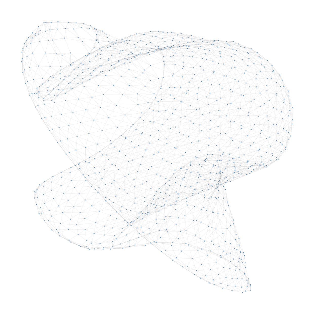
Figure 3: Standard graph visualization: we see the 2d lattice clearly in the connections with a couple longer range correlations crumpling up the graph
Now we need to actually force it into a grid. We can project onto two dimensions using the graph Laplacian whose first two non-trivial eigenvectors should give us coordinates. Because our grid is perfectly square this is only defined up to a rotation so we’ll optimize to find a nice axis-aligned version. We’ll do this with the clean versions to showcase
function embed_coords(C)
    nn = map(1:NPIX) do i
        c = copy(C[:, i]);
        c[i] = -Inf
        Set(partialsortperm(c, 1:k; rev = true))
    end
    g = SimpleGraph(NPIX)
    for i = 1:NPIX, j in nn[i]
        i in nn[j] && add_edge!(g, i, j)
    end
    L = Matrix(laplacian_matrix(g))
    return eigen(Symmetric(L)).vectors[:, 2:3]
end
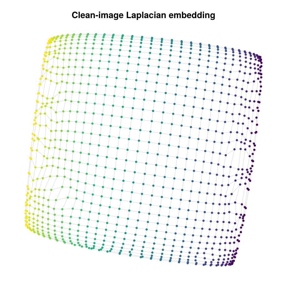
Figure 4: The clean images’ Laplacian embedding, with each pixel joined to its true grid neighbors. Notice our particular issues around the boundaries
Notice that we’re not projecting onto a perfect lattice: the boundaries are tricky due to both boundary conditions as well as the imperfect connections. Both of these induce some distortions we need to deal with. But note that this distortion is a property of the lattice, not of the permutation. Thus the uncorrupted images are distorted in almost the same way. We can use the clean half as a template: we match the clean images’ embedding to our corrupted image embedding (and find the best rotation to match each)
We then only have one final obstacle: the grid looks the same under its eight symmetries (rotations and flips), and local similarity can’t tell them apart. But as you’ll recall from the correlation plot we have some longer range correlations which can help us distinguish better. So we generate all eight orientations of the recovered coordinates and keep the one whose de-corrupted images have a correlation structure closest to that of the genuine originals.
function unscramble(image, orient)
    v = vec(image);
    out = zeros(H, W)
    for i = 1:NPIX
        r, c = orient(rowidx[i], colidx[i])
        out[r, c] = v[i]
    end
    return out
end

function recovered_permutation(orient)
    p = zeros(Int, NPIX)
    for i = 1:NPIX
        r, c = orient(rowidx[i], colidx[i])
        p[i] = r + (c - 1) * H
    end
    return p
end

# Score an orientation by how closely the correlation structure of the
# de-corrupted images matches that of the genuine (non-corrupted) originals.
function orientation_score(orient)
    recovered = [unscramble(img, orient) for img in corrupted_imgs]
    C = cor(flatten(recovered))
    return cor(vec(C), vec(C_orig))     # agreement between the two structures
end
That needs an optimal one-to-one matching between the two point clouds. A greedy nearest-neighbor matching could assign several corrupted pixels to the same clean pixel; we want a true bijection. This is the classic assignment problem, and a compact way to solve it is Bertsekas’ auction algorithm: the clean pixels carry “prices”, each corrupted pixel “bids” for its best-value (nearest) match, contested pixels get more expensive, and prices rise until everyone is matched.
function auction(value)
    n = size(value, 1)
    span = maximum(value) - minimum(value)
    ε = span / 4
    price = zeros(n);
    assign = zeros(Int, n)
    while true
        owner = zeros(Int, n);
        fill!(assign, 0);
        queue = collect(1:n)
        while !isempty(queue)
            i = pop!(queue)
            best = second = -Inf;
            bj = 0
            for j = 1:n
                v = value[i, j] - price[j]
                if v > best
                    second = best;
                    best = v;
                    bj = j
                elseif v > second
                    second = v
                end
            end
            prev = owner[bj]
            prev != 0 && (assign[prev] = 0; push!(queue, prev))
            owner[bj] = i;
            assign[i] = bj
            price[bj] += (best - second) + ε
        end
        ε ≤ span / (4 * n^2) && break
        ε /= 4
    end
    return assign
end

frames = [
    [1 0; 0 1],
    [1 0; 0 -1],
    [-1 0; 0 1],
    [-1 0; 0 -1],
    [0 1; 1 0],
    [0 1; -1 0],
    [0 -1; 1 0],
    [0 -1; -1 0],
]

function match_to_clean(Zc, Zo; iters = 12)
    best_cost, best_assign = Inf, Int[]
    for F in frames
        R = Matrix{Float64}(F);
        assign = Int[]
        for _ = 1:iters
            T = Zo * R'
            dist = sum(Zc .^ 2, dims = 2) .+ sum(T .^ 2, dims = 2)' .- 2 .* (Zc * T')
            assign = auction(-dist)
            U, _, V = svd(Zc' * Zo[assign, :])   # best-fit rotation of the matches
            R = U * V'
        end
        T = Zo * R'
        dist = sum(Zc .^ 2, dims = 2) .+ sum(T .^ 2, dims = 2)' .- 2 .* (Zc * T')
        assign = auction(-dist)
        cost = sum(dist[i, assign[i]] for i = 1:NPIX)
        cost < best_cost && ((best_cost, best_assign) = (cost, assign))
    end
    return best_assign
end
Putting the pieces together: embed both correlation structures, match the corrupted point cloud onto the clean template, read off each corrupted pixel’s recovered grid cell, and finally break the eight-fold symmetry with the orientation score.
Zc = embed_coords(C_perm)
Zo = embed_coords(C_orig)
assign = match_to_clean(Zc, Zo)
rowidx = [cellrow(assign[i]) for i = 1:NPIX]
colidx = [cellcol(assign[i]) for i = 1:NPIX]

dihedral = [ # The eight orientations of a (row, col) assignment.
    (r, c) -> (r, c),
    (r, c) -> (r, W + 1 - c),
    (r, c) -> (H + 1 - r, c),
    (r, c) -> (H + 1 - r, W + 1 - c),
    (r, c) -> (c, r),
    (r, c) -> (c, H + 1 - r),
    (r, c) -> (W + 1 - c, r),
    (r, c) -> (W + 1 - c, H + 1 - r),
]

best = dihedral[argmax(orientation_score.(dihedral))]
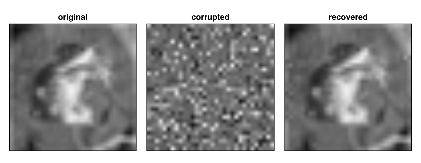
Figure 5: We successfully reconstruct the image!
And we did it! The corrupted image snaps back to something recognizable. We can check the permutation and we find that 1001 / 1024 pixels were recovered to their original position: nearly the whole grid, with the last couple dozen misses being close neighbors on the edges.
Two Permutations: A Further Exercise
This was an excellent interview question. It has a treadmill structure: if candidates are struggling you can spend more time on the first part of the question and probe their knowledge. I’d probably hint strongly about the permutation test and see if the candidate can work out that simpler problem. But for strong candidates who quickly solve the first part we can then move onto the second. The problem with a successful treadmill problem is always the top end: you don’t want to saturate your ability to assess candidates. Lately my strategy to solve this has been to ask the candidate if there’s anything else that comes to mind after I’ve finished the question. Often there’s nothing: they’re just glad to be done. But from time to time they go off in a fascinating new direction that we can explore together. And then I can steal that idea and pose it to the next candidate!
In that spirit I’ll end this post with a further challenge. We’ve currently been working with a single corrupted permutation. Suppose instead we had two corrupted permutations! Can we identify the three sets (original, corrupted with permutation A, corrupted with permutation B)? Note that our permutation test fails: we can’t use it to distinguish between A and B. Enjoy and do let me know if you’ve solved it!
-
You have to listen to her earlier podcast and read her nonfiction and fiction books ↩︎
-
Dwarkesh points out another structure which is that we expect images to have coherent edges while a scrambled image should not. We’ll go with this local consistency first though as we’ll see it’s helpful later: edges are quasi-global which make extracting more information tricky ↩︎